Introduction
Introduction
An isoptic curve of a given plane curve is the locus of points from which the curve is seen under a fixed angle. Equivalently, from any point on the isoptic curve, the two tangent lines drawn to the base curve meet at a prescribed angle.
For a parabola, this construction leads to a surprisingly elegant result: for the viewing angles 45° and 135°, the isoptic locus is a hyperbola. Rotating that planar locus about the axis of symmetry of the parabola then produces the corresponding isoptic surface of the paraboloid of revolution.
This notebook presents the full development in three stages:
◼
derivation of the planar isoptic curve for the parabola ;
y =
2
x
◼
parametrization and animation of the tangent-line geometry;
◼
rotation about the Y axis to obtain the isoptic surface and its associated tangent planes.

1. Deriving the isoptic curve of the parabola
1. Deriving the isoptic curve of the parabola
We begin with the parabola
y=
2
x
and an exterior point from which two tangents are drawn.
(, )
x
0
y
0
Tangent lines from an exterior point
Tangent lines from an exterior point
Obtaining the equations of the tangent lines to a parabola from an outer point:
y-==m(x-);y==+m(x-);-mx+m-==0;
y
0
x
0
y
0
x
0
2
x
x
0
y
0
Due to the condition of tangency:
2
m
x
0
y
0
2
m
x
0
y
0
By Vieta’s theorem:
m
1
m
2
x
m
1
m
2
y
0
Constant-angle condition
Constant-angle condition
The trigonometric identity for the angle between two lines with slopes and is:
m
1
m
2
Tan[α]==-
m
1
m
2
1+
m
1
m
2
For we obtain:
α = 45°
In[]:=
1==-;==;-4==;-16==;Expand[-16==]
m
1
m
2
1+
m
1
m
2
2
(-)
m
1
m
2
2
(1+)
m
1
m
2
2
(+)
m
1
m
2
m
1
m
2
2
(1+)
m
1
m
2
2
(4)
x
0
y
0
2
(1+4)
y
0
2
(4)
x
0
y
0
2
(1+4)
y
0
16-161+8+16;16-16-24-1==0;
2
x
0
y
0
y
0
2
y
0
2
x
0
2
y
0
y
0
Thus the isoptic curve is a hyperbola:
16-16-24y-1==0;
2
x
2
y
Rotating this locus around the Y axis yields the isoptic surface:
16(+)-16-24y-1==0;
2
x
2
z
2
y
This is the isoptic surface of the paraboloid corresponding to the viewing angle 45°.
2. Parametrization of the isoptic curve
2. Parametrization of the isoptic curve
To animate the geometry, it is convenient to rewrite the hyperbola in standard form.
16-16+y+==1-9;16-16==-8;2-2==1;-==1;[t_]:=Sinh[t],±Cosh[t]-;
2
x
2
y
3
2
9
16
2
x
2
y+
3
4
2
y+
3
4
2
x
2
y+
3
4
1
2
2
x
1
2
ζ
iso
2
2
2
2
3
4
So the two branches of the isoptic curve are naturally parametrized by hyperbolic functions.
Slopes of the tangent lines
Slopes of the tangent lines
Obtaining the slopes of the tangent lines to the parabola:
In[]:=
Solve[t]+[t]==4Sinh[t],[t][t]==4-Cosh[t]-,{[t],[t]}
m
1
m
2
2
2
m
1
m
2
2
2
3
4
m
1
m
2
[t][t][t][t]
m
1
2
Sinh[t]-3+2
,2
Cosh[t]+22
Sinh[t]
m
2
2
Sinh[t]+3+2
,2
Cosh[t]+22
Sinh[t]
m
1
2
Sinh[t]+3+2
,2
Cosh[t]+22
Sinh[t]
m
2
2
Sinh[t]-3+2
;2
Cosh[t]+22
Sinh[t]
In[]:=
Solve[t]+[t]==4Sinh[t],[t][t]==4Cosh[t]-,{[t],[t]}
m
11
m
22
2
2
m
11
m
22
2
2
3
4
m
11
m
22
[t][t][t][t]
m
11
2
Sinh[t]-3-2
,2
Cosh[t]+22
Sinh[t]
m
22
2
Sinh[t]+3-2
,2
Cosh[t]+22
Sinh[t]
m
11
2
Sinh[t]+3-2
,2
Cosh[t]+22
Sinh[t]
m
22
2
Sinh[t]-3-2
;2
Cosh[t]+22
Sinh[t]
3. Animation of the planar isoptic curve
3. Animation of the planar isoptic curve
The next interactive figure shows the parabola, the two branches of its isoptic curve, and the corresponding tangent pairs. As the marked point moves, the angle between the tangent lines remains constant along each branch.
Manipulate[t_]:=[t_]:=[t_]:=[t_]:=};[t_]:=Sinh[t],Cosh[t]-;[t_]:=Sinh[t],-Cosh[t]-;Show[{ParametricPlot[ζ[t],{t,-6,6},PlotStyle{Blue,Thick}],ParametricPlot[[t],{t,-2,2},PlotStyle->Red,MaxRecursion->3],ParametricPlot[[t],{t,-2,2},PlotStyle->Red,MaxRecursion->3],Plot[[t1][[2]]+[t1](x-[t1][[1]]),{x,-6,6},PlotStyle->{Black,Thick}],Plot[[t1][[2]]+[t1](x-[t1][[1]]),{x,-6,6},PlotStyle->{Black,Thick}],Plot[[t1][[2]]+[t1](x-[t1][[1]]),{x,-6,6},PlotStyle->{Green,Thick}],Plot[[t1][[2]]+[t1](x-[t1][[1]]),{x,-6,6},PlotStyle->{Green,Thick}],Graphics[{Black,PointSize[0.01],Point[[t1]],Text[Style["P",14,Bold],[t1],{0,-1.2}],Point[[t1]],Text[Style["",14,Bold],[t1],{0,-1.2}]}]},AspectRatioAutomatic,AxesTrue,AxesOrigin{0,0},AxesLabel{x,y},PlotRange6,ImageSize700],Style["Isoptic curve of a parabola",Bold,Large],{{t1,-2+0.00002,"Value (t1)"},-2+0.00001,2,0.00001},ControlPlacementTop
m
1
2
Sinh[t]-3+2
;2
Cosh[t]+22
Sinh[t]
m
2
2
Sinh[t]+3+2
;2
Cosh[t]+22
Sinh[t]
m
11
2
Sinh[t]-3-2
;2
Cosh[t]+22
Sinh[t]
m
22
2
Sinh[t]+3-2
;ζ[t_]:={t,2
Cosh[t]+22
Sinh[t]
2
t
ζ
iso
2
2
2
2
3
4
ζ
iso1
2
2
2
2
3
4
ζ
iso
ζ
iso1
ζ
iso
m
11
ζ
iso
ζ
iso
m
22
ζ
iso
ζ
iso1
m
1
ζ
iso1
ζ
iso1
m
2
ζ
iso1
ζ
iso
ζ
iso
ζ
iso1
P
1
ζ
iso1
Out[]=


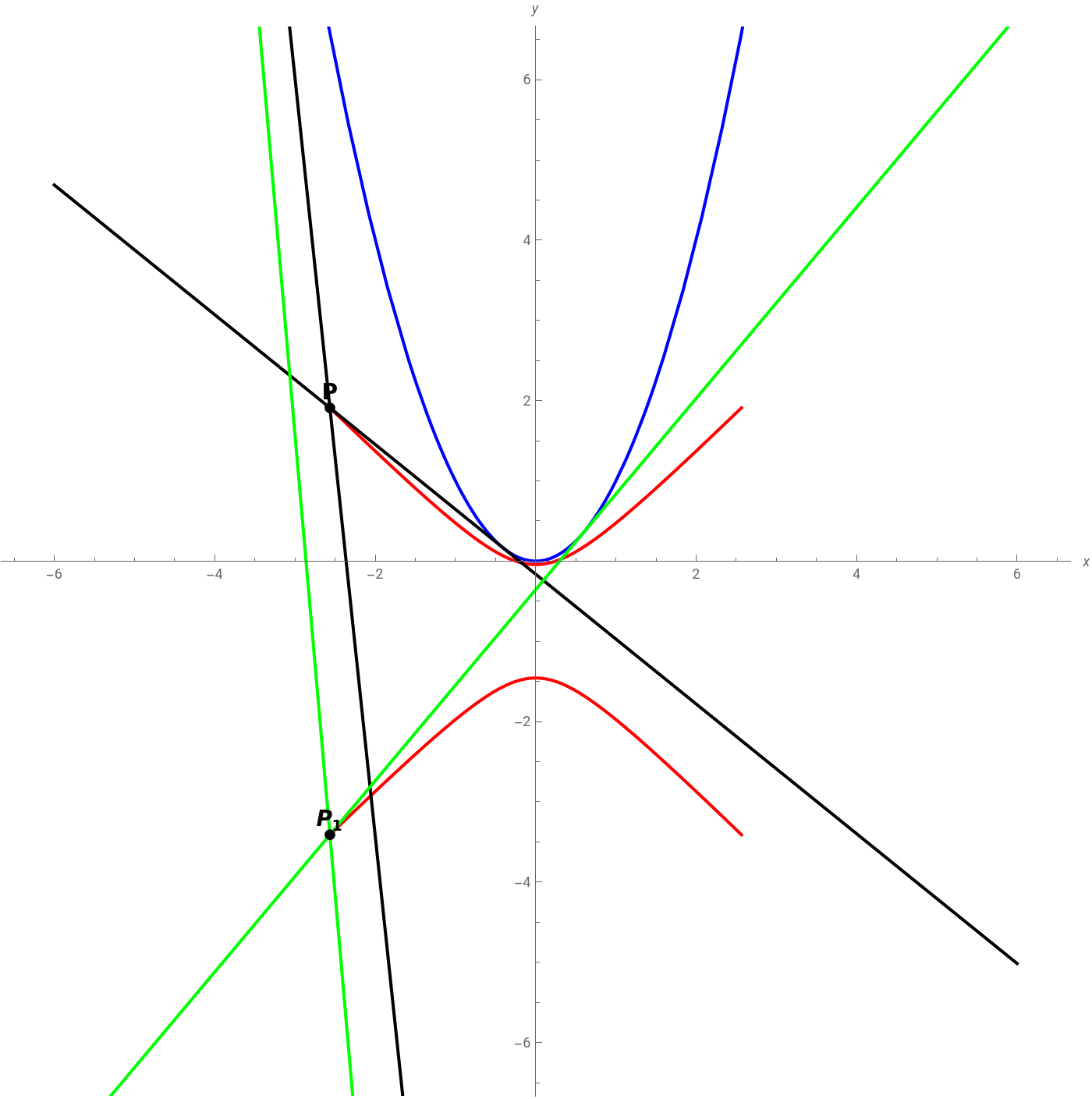
When the intersection point lies below the X axis, the tangent angle is 45°; when it lies above, the angle is 135°.
4. Rotating the isoptic curve: the isoptic surface of the paraboloid
4. Rotating the isoptic curve: the isoptic surface of the paraboloid
The isoptic surface is obtained by revolving the planar isoptic curve about the Y axis, exactly as the parabola itself generates the paraboloid of revolution.
This visualization makes the rotational symmetry of the construction especially clear.
5. Motion of the tangent planes along the isoptic surface
5. Motion of the tangent planes along the isoptic surface
Each point of the isoptic surface determines a pair of tangent planes to the paraboloid meeting at the prescribed angle. The following animation shows how those tangent planes move as the point rotates around the axis.
6. Why only pairs of tangent planes?
6. Why only pairs of tangent planes?
The configuration of three tangent planes through a point occurs only in the orthoptic case, where one seeks tangent planes that are mutually perpendicular. For a paraboloid, the locus from which three pairwise orthogonal tangent planes can be drawn is the Monge plane.
For any angle other than 90°—in particular for 45° and 135°—the isoptic property is determined by pairs of tangent planes, not triples.
The tangent planes to the paraboloid therefore take the form
Interpreting the coefficient of x
Interpreting the coefficient of x
Then
For 45°:
For 135°:
This explains the coefficients multiplying x in the tangent-plane equations.
7. Derivation of the isoptic radii
7. Derivation of the isoptic radii
Let
Take the plane
whose normal vector is
Substituting into the plane equation yields the radius:
Conclusion
Conclusion
The geometry of isoptic loci reveals a beautiful connection between tangency, constant-angle viewing, and surfaces of revolution. In this case:
◼
rotating that curve about the Y axis gives the isoptic surface of the paraboloid;
◼
each point on the resulting surface determines a pair of tangent planes meeting at the prescribed angle.
The constructions shown here illustrate how a planar constant-angle condition naturally extends into three-dimensional geometry through rotational symmetry.