We first analyze the halting times of 2-state 2-color Turing Machines and classify them. We then create and visualize the multiway graph formed by generating 2-state Busy Beaver candidates using the Tree Normal Form method. Next, we analyze advanced techniques to speed up the simulation of arbitrary Turing Machines: first, by building stackable multi-symbol Macro Machine Turing Machines, and second, by implementing an “exponential form” for the tape whose primary benefit is eliminating repetition. We end by exploring automated proof generation machines, a functionality built on top of both Macro Machines and exponential form which automates the task of inductive proof on tape configurations.
Introduction
Introduction
Imagine you have a magical tape.
On this tape, you can perform any computation you desire, from calculating the next prime number to solving Sudoku. This isn’t just any tape—it’s the theoretical foundation of all modern computers, the Turing Machine. Conceptualized by Alan Turing, this abstract device might not look impressive at first glance—just a tape, a head, and a set of rules. But despite its deceptively straightforward design, it’s like the Swiss Army knife of computation, capable of solving an infinite array of diverse problems with a finite set of rules.
A Turing Machine operates on an infinite tape divided into cells, each containing a symbol. It has a head that reads and writes symbols on the tape according to a table of rules. Remarkably, any algorithm can be simulated by a Turing Machine, which is why the standard benchmark for new programming languages is Turing-completeness.
Busy Beaver candidates are a particularly interesting subclass of Turing Machines, where one state is deemed a “halting” state — a state where the Turing Machine simply stops running. The machine of this kind which runs for the longest amount of time before stopping is called the Busy Beaver champion. It turns out that studying the halting times of these kinds of machines reveals insights about both math and the limits of computation.
In this project, we’ll explore the complex world of Busy Beaver candidates, focusing on their halting times. We answer three core questions: How can we efficiently find Busy Beavers? How can we quickly simulate Turing Machines? And can we automate the task of proof writing?
On this tape, you can perform any computation you desire, from calculating the next prime number to solving Sudoku. This isn’t just any tape—it’s the theoretical foundation of all modern computers, the Turing Machine. Conceptualized by Alan Turing, this abstract device might not look impressive at first glance—just a tape, a head, and a set of rules. But despite its deceptively straightforward design, it’s like the Swiss Army knife of computation, capable of solving an infinite array of diverse problems with a finite set of rules.
A Turing Machine operates on an infinite tape divided into cells, each containing a symbol. It has a head that reads and writes symbols on the tape according to a table of rules. Remarkably, any algorithm can be simulated by a Turing Machine, which is why the standard benchmark for new programming languages is Turing-completeness.
Busy Beaver candidates are a particularly interesting subclass of Turing Machines, where one state is deemed a “halting” state — a state where the Turing Machine simply stops running. The machine of this kind which runs for the longest amount of time before stopping is called the Busy Beaver champion. It turns out that studying the halting times of these kinds of machines reveals insights about both math and the limits of computation.
In this project, we’ll explore the complex world of Busy Beaver candidates, focusing on their halting times. We answer three core questions: How can we efficiently find Busy Beavers? How can we quickly simulate Turing Machines? And can we automate the task of proof writing?
The Behavior of [2,2] Turing Machines
The Behavior of [2,2] Turing Machines
Turing Machines grow faster than any computable function. Because of this, it is often logistically infeasible to print out the output of even a decently sized Turing machine.
Therefore, to study these creatures, we first start with something much easier: Turing Machines with two head states (states and ) and two cell states (0 and 1). The word “state” is usually reserved for the head state, while “color” or “symbol” is used for the cell state. We’ll refer to a 2-state 2-color Turing Machine as a [2, 2] TM, and in general, a -state -color Turing Machine is abbreviated as [n, k].
Therefore, to study these creatures, we first start with something much easier: Turing Machines with two head states (states
1
2
n
k
Generating all 2048 [2,2] Machines
Generating all 2048 [2,2] Machines
2-state 2-color TMs have four rules: one for every combination of state and color. As an example, if the TM is in state 1 and sees a 0, corresponding to the input {1, 0}, it will do three things:
1
.Change its head state,
2
.Write down a symbol, overriding the one it currently sees,
3
.Move left or right.
This information is encapsulated in a rule: given a input state and symbol, return a new state, what to write in the cell, and which direction to move. This is the fundamental structure of a Turing Machine: a list of rules.
Of these rules, one is special: it encodes a “halt” command. We reserve a state dedicated to the “halt” state.
Definition. The “halt” state of a n-state 2-color Busy Beaver Turing Machine is defined as state n+1. For example, for 2-state machines, state 3 is the halt state. We will use this notation throughout the rest of the notebook, so we can generalize past 2-state TMs.
Of these rules, one is special: it encodes a “halt” command. We reserve a state dedicated to the “halt” state.
Definition. The “halt” state of a n-state 2-color Busy Beaver Turing Machine is defined as state n+1. For example, for 2-state machines, state 3 is the halt state. We will use this notation throughout the rest of the notebook, so we can generalize past 2-state TMs.
Busy Beaver Numbers
Busy Beaver Numbers
Before we begin to explore, we will first define some terms:
Definition. The n-state Busy Beaver is the [n, 2] Turing Machine which runs for at least as many steps before stopping as any other [n, 2] Turing Machine.
Note how we define it as “at least as many,” as there are sometimes multiple n-state Busy Beavers which each run for the same duration.
Definition. is equal to the amount of 1s left over by a n-state Busy Beaver.
A more natural sequence that can measure what the “productivity” of a terminating machine is:
Definition. is equal to the greatest number of steps that can be performed by a n-state 2-color Turing machine which eventually halts.
Authors are conflicted on whether to define or as the nth Busy Beaver number. We think that is a more natural definition, as we expect most readers will agree. Thus, we will refer to the sequence as “the Busy Beaver numbers” and as “the nth Busy Beaver number.”
Definition. The n-state Busy Beaver is the [n, 2] Turing Machine which runs for at least as many steps before stopping as any other [n, 2] Turing Machine.
Note how we define it as “at least as many,” as there are sometimes multiple n-state Busy Beavers which each run for the same duration.
Definition.
Σ(n)
A more natural sequence that can measure what the “productivity” of a terminating machine is:
Definition.
S(n)
Authors are conflicted on whether to define
Σ(n)
S(n)
S(n)
S
S(n)
Defining Shorthand Functions
Defining Shorthand Functions
Wolfram Language has built-in functions for both the creation of a Turing Machine and the visualization of a machine’s output.
In[]:=
exampleTuringMachine=TuringMachine[{{1,0}{2,1,1},{1,1}{3,0,0},{2,0}{2,1,-1},{2,1}{1,1,-1}}];
Notice that the third index in the output list of nearly all rules is either a or a . A corresponds to “move right”, corresponds to “move left”. However, halt states always have as its third item.
Let’s plot out the output of this Turing Machine for ten steps:
1
-1
1
-1
0
Let’s plot out the output of this Turing Machine for ten steps:
In[]:=
RulePlot[exampleTuringMachine,{1,{{},0}},10]
Out[]=

What does this graph mean? Each row displays the relevant part of the infinite tape — i.e. all cells which the tape head has ever reached. The y-axis is time, measured in steps: the upper row shows “time 0”, when zero steps have been performed. The head’s direction corresponds to the head state: looking directly up is state 1, looking towards bottom right is state 2, and bottom left is state 3 (halt).
Both the code for the creation for a Turing Machine and seeing the plot of it is fairly long right now. Due to this, we create some shorthand functions:
Both the code for the creation for a Turing Machine and seeing the plot of it is fairly long right now. Due to this, we create some shorthand functions:
In[]:=
TM[rules_List] := TuringMachine[rules]TM[rules_List, steps_Integer] := TuringMachine[rules, {1, {{}, 0}}, steps]TMP[rules_List, steps_Integer : 15] := RulePlot[TM[rules], {1,{{}, 0}}, steps] (*"Turing Machine Plot"*)TMP[rules_List, steps_Integer : 15, pixels_Integer] := RulePlot[TM[rules], {1,{{}, 0}}, steps, ImageSize -> {Automatic, pixels}]
Rule Generation
Rule Generation
Writing out individual TM instructions is painfully tedious. Instead, we can generate them by analyzing the fundamental structure of a Turing Machine. As we stated before, a TM consists of a set of rules, and a [2,2] TM has four rules. But what does a rule look like? Take this example:
In[]:=
exampleRule={2,0}{2,1,-1};
In general, a rule looks like . For 2-state 2-color TMs, we have that and , so we can generate all the possible inputs with
{inputState,inputSymbol}->{newState,cellWrite,moveDirection}
1<=inputState<=2
inputSymbol={0,1}
In[]:=
Flatten[Table[{inputState,inputSymbol},{inputState,1,2},{inputSymbol,0,1}],1]
Out[]=
{{1,0},{1,1},{2,0},{2,1}}
Similarly, we can use nested variables inside a to generate the possible outputs; however, we must also include the halting state , as so:
Table
{3, 0, 0}
In[]:=
Flatten[Table[{nextState,cellWrite,headMove},{nextState,1,2},{cellWrite,0,1},{headMove,{-1,1}}],2]//Append[{3,0,0}]
Out[]=
{{1,0,-1},{1,0,1},{1,1,-1},{1,1,1},{2,0,-1},{2,0,1},{2,1,-1},{2,1,1},{3,0,0}}
Now we iterate over all possible mappings from to four outputs from :
allInputs
allOutputs
In[]:=
Module[{headStates, transitions, haltingTransition, transitionLists}, haltingTransition = {3, 0, 0}; (*State 3 is reserved for a halting state*) headStates = Flatten[Table[{i, j}, {i, 1, 2}, {j, 0, 1}], 1]; (*all possible inputs for a [2,2] Turing Machine*) transitions= Flatten[ Table[ {nextState, cellWrite, headMove} ,{nextState, 1, 2} ,{cellWrite, 0, 1} ,{headMove, {-1, 1}} ] ,2] // Append[haltingTransition]; (*all possible outputs*) transitionLists = Tuples[transitions, {Length[headStates]}] // Select[Count[haltingTransition] /* EqualTo[1]]; (*only selecting tuples with exactly 1 halting output*) busyBeavers2 = Table[Thread[headStates -> transitionList], {transitionList, transitionLists}];]
We keep all the [2,2] Turing Machines in a list called : these are the candidates for the 2-state Busy Beaver. There are 2048 candidates, which we can quickly verify with
busyBeavers2
In[]:=
busyBeavers2//Length
Out[]=
2048
If we want to get a flavor for the behavior of a certain Turing Machine, we can use our shorthand functions from before alongside :
busyBeavers2
In[]:=
Column[{" Behavior of [2,2] Turing Machine #1121 ",RulePlot[TM[busyBeavers2[[1321]]]],TMP[busyBeavers2[[1321]],25]},Frame->True,Alignment->Center]
Out[]=
Behavior of [2,2] Turing Machine #1121 |
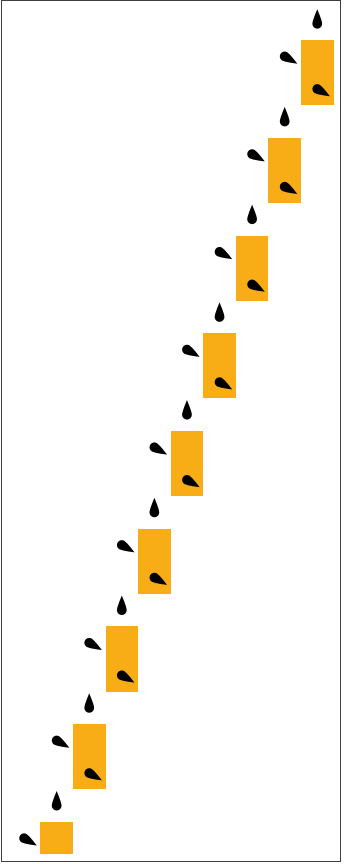
where the legend is above the output of the TM. In the rule legend, the upper box represents the input configuration, and the lower box represents the output configuration, with the offset being the head movement.
Let’s wrap this in a and iterate over all the [2,2] Turing Machines:
Let’s wrap this
Column
Manipulate
In[]:=
Manipulate[Column[{" Behavior of [2,2] Turing Machine #"<>ToString[index]<>" ",RulePlot[TM[busyBeavers2[[index]]]],TMP[busyBeavers2[[index]],25]},Frame->True,Alignment->Center],{index,1,Length[busyBeavers2],1},ControlType->Slider,SaveDefinitions->True]
Out[]=

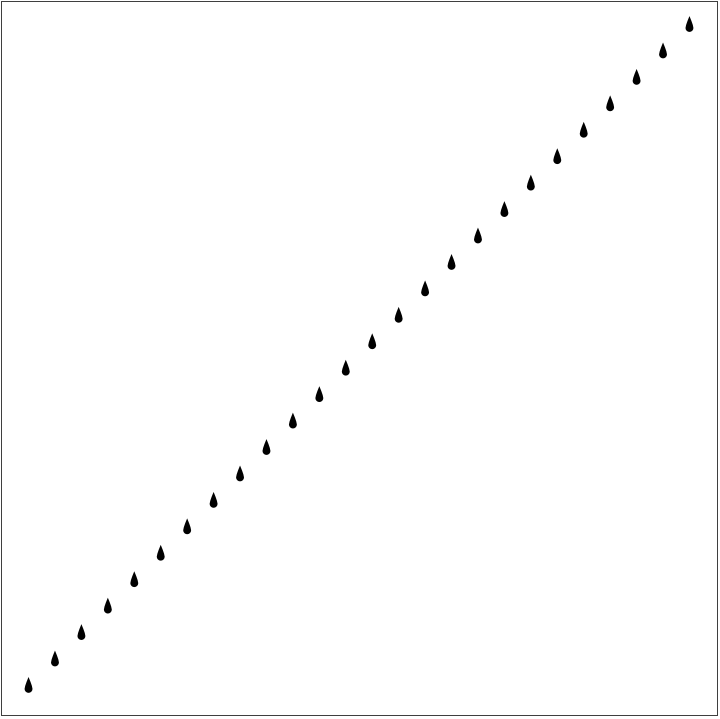
The first thing we notice is that a sizeable portion of the 2048 Turing Machines aren’t that interesting. In fact, the first 776 TMs display very simple behavior: going infinitely on in one direction of the tape. From just looking at these plots, we can make educated guesses about whether they halt or not. But what if we want to do better than an educated guess?
To Halt or Not To Halt
To Halt or Not To Halt
The halting problem is a famous decision problem which asks, “given an arbitrary Turing Machine, can you always correctly predict if it halts?” In 1936, Alan Turing published a proof by contradiction showing that no, it is impossible. Does this mean that the pursuit of finding Busy Beaver numbers is pointless?
Of course not. There’s a lot more computation left in this essay, after all. While it is impossible to create a infinitely smart machine that can always tell whether a Turing Machine halts, researchers have still found quite a few ways to determine whether a Turing Machine terminates. We go over two basic ways in this section.
Of course not. There’s a lot more computation left in this essay, after all. While it is impossible to create a infinitely smart machine that can always tell whether a Turing Machine halts, researchers have still found quite a few ways to determine whether a Turing Machine terminates. We go over two basic ways in this section.
The Genie in the Bottle: Busy Beaver Numbers
The Genie in the Bottle: Busy Beaver Numbers
One reason why Busy Beaver numbers are so important is that if the nth Busy Beaver number is known, then we can easily determine whether any [n, 2] Turing Machine halts. Consider the following algorithm to determine whether a n-state 2-color TM halts:
2
.If it halts, it halts. If it hasn’t, it won’t.
We can see that most machines never terminate, with less halting machines that survive for longer. This makes sense. The Busy Beavers, the most productive machines that take the longest to halt, are also much rare than machines which halt after one step.
If we want to see which beavers are the most productive, we can sort our comprehensive list of all possible rules and sort them based on how long they halt and if they halt:
If we want to see which beavers are the most productive, we can sort our comprehensive list of all possible rules and sort them based on how long they halt and if they halt:
If so simple, why not use this method all the time? Because finding Busy Beaver numbers is difficult and impossible past a certain point. Proving the value of the fifth Busy Beaver number alone was a task that took over four decades to complete, with the end proof being published only a week before this essay was published.
Here is a chart on how long it took to find and prove Busy Beaver numbers:
Here is a chart on how long it took to find and prove Busy Beaver numbers:
This number is so big that the number of digits in it is greater than the number of atoms in the observable universe, and even the number of digits in the number of digits of that number is still greater. To begin to approach determining whether machines such as that machine halt or not, we will need more sophisticated techniques than simply running the machine for a long time.
Road Runners
Road Runners
With this in hand, we can use pattern checking alongside our helper functions to write a better simplisticRoadRunnerQ:
This should catch all 26 remaining TMs which do not halt but also are not road runners.
Indeed, it does!
Neat visualizations of TMs
Neat visualizations of TMs
Let’s see what these graphs look like:
Looking at the graphs for road runners gives us a more intuitive understanding of why they halt. Take the graph of Busy Beaver #258:
Because state 1 loops back into itself on input symbol 0, it goes on infinitely to the right without writing anything. Indeed, we can see from the plot, it does go on infinitely:
Tree Normal Form
Tree Normal Form
Background
Background
What’s the issue with our earlier rule generation?
What’s the issue with our earlier rule generation?
While it is fast enough to generate all the 2048 [2,2] TMs with our nested list rule generation, it quickly becomes infeasible. The problem is that an overwhelming majority of machines are redundant; for example, if the first state maps to the halt state, then none of the other state transitions matter. If there was some way to reduce this redundancy, that would be useful...
How TNF Works
How TNF Works
Once this TM runs for one step and realizes that it is running an “unwritten” rule, it branches off, with each branch representing a different possible rule for that unwritten rule.
In other words, at each step, each edge is like writing one more rule. Therefore, TMs that are a greater number of edges away are more “complete,” and the TMs that are furthest from the origin are usually where we find Busy Beavers.
Meanwhile, this algorithm spares a lot of repetition in terms of non-terminating or quickly-terminating machines. Machines that terminate or are determined to run infinitely and not hit a “unwritten” rule are left alone and are leaf nodes, even if they don’t have all their rules written.
In other words, at each step, each edge is like writing one more rule. Therefore, TMs that are a greater number of edges away are more “complete,” and the TMs that are furthest from the origin are usually where we find Busy Beavers.
Meanwhile, this algorithm spares a lot of repetition in terms of non-terminating or quickly-terminating machines. Machines that terminate or are determined to run infinitely and not hit a “unwritten” rule are left alone and are leaf nodes, even if they don’t have all their rules written.
Implementing Tree Normal Form for [2,2] TMs
Implementing Tree Normal Form for [2,2] TMs
TNF in Tree form
TNF in Tree form
Wow. That’s quite a compact image. Is there any way we can visualize it in a nicer fashion?
TNF as a multiway graph rule
TNF as a multiway graph rule
Let’s take a second to observe the graph. Looking at the generation of [2, 2] Turing Machines this way unveils (or makes clearer) a few interesting properties:
◼
The further away from the origin, the more machines halt. As a corollary, all Busy Beavers can be found on the very perimeter.
◼
Tree Normal Form rule generation avoids the thousands of road runners that nested list rule generation does. In fact, the total number of vertices is
We wish to see how many of these machines still lead to a “unwritten” state, which of these machines halt, and which never halt. To do this we create a classifier:
which we then use to analyze all the vertices:
Expansion to 3-state Turing Machines
Expansion to 3-state Turing Machines
As promised, we are no longer limited to [2, 2] TMs. To add one more state to become a 3-state 2-color TM, we need a new “blank slate” Turing Machine:
Still handle-able so far. The number of vertices is only 118:
Troubles start to arise with a depth of 3:
There are now 794 vertices:
Notice how the number of nodes is the same at a depth of 7 as a depth of 6. This is because a 3-state 2-color Turing Machine has six total rules, and since each edge away from the origin writes one rule, all the Turing Machines at a depth of six from the initial blank state are fully written. In other words, there are no depth 7 nodes.
This analysis only scratches the surface of the multiway graphs birthed from applying Tree Normal Form — though we can already see the strength it demonstrates in limiting the Turing Machine search space.
Advanced Simulation Techniques
Advanced Simulation Techniques
Macro Machines: Turing Machine Inception
Macro Machines: Turing Machine Inception
How it works (part 1)
How it works (part 1)
Note that while we only used a block size of 3 in our example, it is very easy to generalize to greater size chunks. However, we must remember that the number of symbols is exponentially tied to the size of the chunk. Generating a 10-chunk Macro Machine on top of a simple 2-state 2-color Turing Machine would create a 4-state 1024-color Macro Machine.
How it works (part 2)
How it works (part 2)
Now for the transitions. Each transition takes in a input state with an orientation and a finite section of tape, and we must run our original TM on it until it leaves. This is straightforward. But there is trick hidden here: Until it leaves. What if it never does?
We must also consider two edge cases:
We must also consider two edge cases:
1
.The tape head enters an infinite cycle within the 3-block symbol.
2
.The tape head halts within the 3-block symbol.
And let’s double check that they’re the same:
Amazing! It works.
Speed analysis
Speed analysis
Generalizing informedHaltsQ and transitionGraph
Generalizing informedHaltsQ and transitionGraph
Further, since Macro Machine graphs typically get quite large, we will (1) make “HALT” transitions red to stand out and (2) add the option to remove edge labels. All combined, our transition function becomes:
With these functions, we can easily create an analogous animation of all 2048 [2, 2] Turing Machines — all 2048 Macro Machines generated from those Turing Machines:
Busy Beavers!
Busy Beavers!
It’s been over two full sections and we still haven’t looked at the namesake of this essay: Busy Beavers. The machines we alluded to at the very beginning, who run for longer before halting than any other machine with the same number of states. Here, we will observe the 3rd, 4th, and 5th Busy Beaver machines.
Three-state Winner
Three-state Winner
Changing the way we view the tape
Changing the way we view the tape
Exponent Tape Notation
Exponent Tape Notation
We can check whether this exponential tape notation actually works by running our 2048 Macro Machines on top of it from earlier:
Nice.
Opening the door for automated proof generation
Opening the door for automated proof generation
Now comes the question of how to actually prove an inductive hypothesis. Above, we discussed one case: that two tapes would differ only in their exponents, and their bases would all match. In this case, we can run a macro machine with arbitrary exponents w, x, y, z, ... until we either transform the tape into the inductive form we wish, or fails. If it succeeds, the proof machine keeps that proof in a database, which it can now access at any point.
Another possibility is if not all the bases match. In these cases, it may be harder to form an inductive proof. But in many cases, the exponents will give away important info; for example, if the maximum exponent of any base in the tape goes {1, 2, 5, 5, 8, 16, 32, 64, 128, ...} we can tell that there is likely a proof to be written with exponent powers of two. The Macro Machine and exponent tape functions above provide the groundwork for this kind of algorithm, opening the door for a proof machine.
Another possibility is if not all the bases match. In these cases, it may be harder to form an inductive proof. But in many cases, the exponents will give away important info; for example, if the maximum exponent of any base in the tape goes {1, 2, 5, 5, 8, 16, 32, 64, 128, ...} we can tell that there is likely a proof to be written with exponent powers of two. The Macro Machine and exponent tape functions above provide the groundwork for this kind of algorithm, opening the door for a proof machine.
Conclusion
Conclusion
We can’t catch ‘em all — no matter how wide a net we cast, it is certain that a number of Busy Beaver machines will always have to be checked by hand. But for the first few Busy Beaver numbers, we can relatively simply (though it costs great computational power) generate them and analyze their halting times given the appropriate Busy Beaver number. If not given S(n), we can detect with high accuracy whether a machine immediately enters an infinite loop with smarterRoadRunnerQ. A good visualization (which automatically prunes clearly unnecessary machines) is Tree Normal Form, which also can generate a multiway graph. We next looked at Macro Machines, a “higher-level” Turing Machine built on top of a regular TM which speeds up the process of brute-force simulation. Further speeding this process up is exponent notation, which eliminates the worst form of repetition. The idea of an automated proof machine is discussed in the final section.
Further Research
Further Research
Acknowledgements
Acknowledgements
My mentor Dugan Hammock provided constant support and patience, and always gave advice which sparked a new path to explore. Tyler Rose helped debug various functions in this project. Stephen Wolfram gave me the initial idea. All the TAs, mentors, and directors made Wolfram Summer Research Program an excellent two weeks. I am thankful and indebted to them all for making the completion of this project possible.
Bibliography
Bibliography
◼
Brubaker, Ben. “Amateur Mathematicians Find Fifth “Busy Beaver” Turing Machine.” Quanta Magazine, 2 July 2024, www.quantamagazine.org/amateur-mathematicians-find-fifth-busy-beaver-turing-machine-20240702/. Accessed 11 July 2024.
◼
Harland, James. “Analysis of Busy Beaver Machines via Induction Proofs.” Computing: The Australasian Theory Symposium, 30 Jan. 2007, crpit.scem.westernsydney.edu.au/confpapers/CRPITV65Harland.pdf. Accessed 11 July 2024.
◼
Holkner, Alex. Acceleration Techniques for Busy Beaver Candidates. Jan. 2004, www.researchgate.net/publication/254389437_ACCELERATION_TECHNIQUES_FOR_BUSY_BEAVER_CANDIDATES. Accessed 11 July 2024.
◼
Ligocki, Shawn. “BB(6, 2) > 10↑↑15.” Sligocki, 21 June 2022, www.sligocki.com/2022/06/21/bb-6-2-t15.html. Accessed 11 July 2024.
◼
Marxen, Heiner. “Heiner Marxen - Macro Machines.” Turbotm.de, 11 June 2010, turbotm.de/~heiner/BB/macro.html. Accessed 11 July 2024.
◼
Weisstein, Eric W. “Busy Beaver.” Mathworld.wolfram.com, mathworld.wolfram.com/BusyBeaver.html. Accessed 11 July 2024.
◼
Wolfram, Stephen. “Multiway Turing Machines—Wolfram Physics Bulletins.” Www.wolframphysics.org, 4 Feb. 2021, www.wolframphysics.org/bulletins/2021/02/multiway-turing-machines/. Accessed 11 July 2024.
◼
Yedidia, Adam, and Scott Aaronson. A Relatively Small Turing Machine Whose Behavior Is Independent of Set Theory. 13 May 2016, arxiv.org/pdf/1605.04343, https://doi.org/10.48550/arXiv.1605.04343. Accessed 11 July 2024.
CITE THIS NOTEBOOK
CITE THIS NOTEBOOK
Generating macro machine simulations and proofs of halting for busy beaver Turing machines
by Owen Xuan
Wolfram Community, STAFF PICKS, July 12, 2024
https://community.wolfram.com/groups/-/m/t/3216803
by Owen Xuan
Wolfram Community, STAFF PICKS, July 12, 2024
https://community.wolfram.com/groups/-/m/t/3216803