This Project attempts to provide a thorough implementation of the system of Tree Calculus in the wolfram language, including tools for producing, visualizing, and evaluating Tree Calculus programs. Tree Calculus is a low level functional model of computation introduced by Barry Jar. The programs of tree calculus are entirely composed of the self-application of a single ternary operator. Unlike many similar models, such as Turing Machines or Lambda Calculus, Tree Calculus does not require named variables. This allows for programs to be fully represented as unlabeled binary trees, leading to the name Tree Calculus. In addition to being more fundamental than other similar models of computation, Tree Calculus is in a sense more powerful, allowing for programs that can compute their own size, determine their own equality, or self-evaluate, all without the need for any for of external machinery. This project will lay out the rules governing Tree Calculus, provide examples of how important functions are represented in Tree Calculus, and demonstrate the power of tree calculus through reflective programs
Definitions
Definitions
Initialization
Fundamental Definitions
Fundamental Definitions
Definition of the Node function
Definition of the Node function
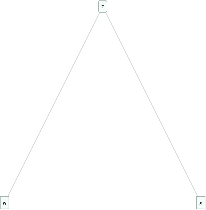
The node function - represented by either Node or Δ - is defined by three rules that determine its behavior depending on the structure of its first argument.
In[]:=
reduceRules={Node[Node,y_,z_]->y,Node[Node[x_],y_,z_]->(y[z])[x[z]],Node[Node[w_,x_],y_,z_]->z[w,x]}
Out[]=
{Δ[Δ,y_,z_]y,Δ[Δ[x_],y_,z_]y[z][x[z]],Δ[Δ[w_,x_],y_,z_]z[w,x]}
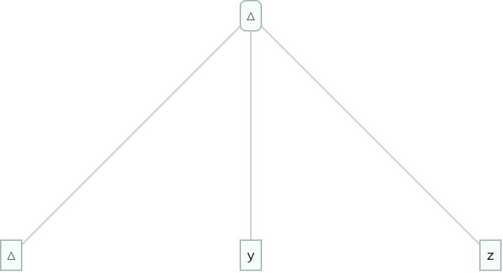
The Kernel Rule
In[]:=
ExpressionTree[Node[Node,y,z]]->ExpressionTree[y]
Out[]=

The Stem Rule
In[]:=
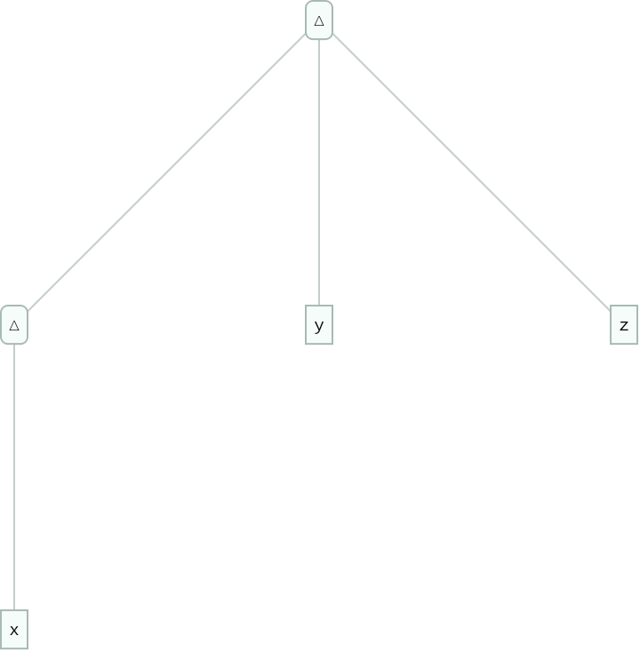
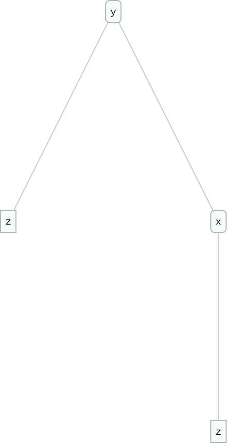
ExpressionTree[Node[Node[x],y,z]]->ExpressionTree[y[z,x[z]]]
Out[]=
The Fork Rule
In[]:=
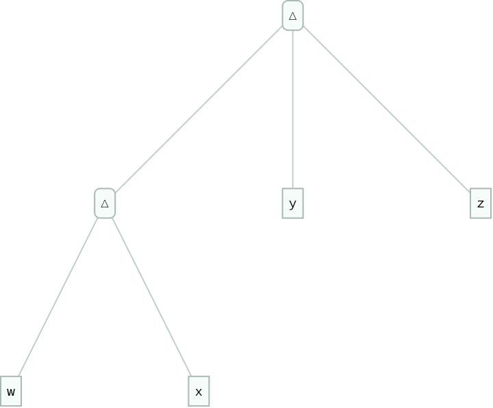
ExpressionTree[Node[Node[w,x],y,z]]->ExpressionTree[z[w,x]]
Out[]=
These definitions quickly lead to representations of the basic combinators
In[]:=
cK=Node[Node];(*K[x,y]=x*)
In[]:=
cI=Node[Node[Node],Node[Node]];(*I[x]=x*)
In[]:=
cD=Node[Node[Node],Node[Node,Node]];(*D[x,y,z]=y[z][x[z]]*)
In[]:=
d[x_]:=Node[Node[x]](*shorthandforthereducedformofD[x]*)
In[]:=
cS=d[cK[cD]][d[cK][cK[cD]]];(*S[x,y,z]=x[z][y[z]]*)
Boolean
Boolean
The definitions of True and False are equivalent to the way they are defined in Lambda calculus
In[]:=
cTrue=Node[Node];(*True[x,y]=x*)
In[]:=
cFalse=Node[Node,Node[Node[Node],Node[Node]]];(*False[x,y]=y*)
With minimal effort, we get definitions of all basic boolean functions
In[]:=
cAnd=d[cK[cK[cI]]];cOr=d[cK[cK]][cI];cNot=d[cK[cK]][d[cK[cK[cI]]][cI]];
In[]:=
cImplies=d[cK[cK]];cIFF=Node[Node[cI,cNot],Node];
Numerical
Numerical
Definition of the natural numbers
In[]:=
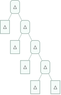
cN[n_Integer]:=Nest[cK,Node,n]
As an example, 4 is represented as:
This leads to relatively simple definitions of the successor and predecessor functions
In[]:=
cSucc=cK;
In[]:=
cPred=d[cK[cK[cI]]][d[cK[Node]][Node]];
Fundamental Queries
Fundamental Queries
This trio of functions provide the foundation for programs capable of examining the structure of other programs
In[]:=
cQuery[a_,b_,c_]:=d[cK[b]][d[cK[cK[cI]]][d[Nest[cK,c,5]][d[cK[cK[cK[a]]]][Node]]]]
In[]:=
cIsLeaf=cQuery[cK,cK[cI],cK[cI]];
In[]:=
cIsStem=cQuery[cK[cI],cK,cK[cI]];
In[]:=
cIsFork=cQuery[cK[cI],cK[cI],cK];
Extensional
Extensional
The below function provides the most simple example of recursion in tree calculus.
It applies the given function to itself, ie. SelfApply[x]=x[x]
Thus, if Y is applied to itself, SelfApply[SelfApply] simplifies into SelfApply[SelfApply], creating a recursive loop.
It applies the given function to itself, ie. SelfApply[x]=x[x]
Thus, if Y is applied to itself, SelfApply[SelfApply] simplifies into SelfApply[SelfApply], creating a recursive loop.
In[]:=
cSelfApply=d[cI][cI];
We define a series of functions that hold one or more functions from evaluating until further input is received, allowing for recursion to be prevented until a desired point.
In[]:=
cWait[x_,y_]:=d[cI][d[cK[y]][cK[x]]]
In[]:=
cWait1[x_]:=d[d[cK[cK[x]]][d[d[cK][cK[Node]]][cK[Node]]]][cK[d[Node[cK,cK]]]]
In[]:=
cWait2[x_,y_]:=d[d[cK[d[cK[y]][cK[x]]]][d[d[cK][cK[Node]]][cK[Node]]]][cK[d[cI]]]
These functions can be combined to create the Tree Calculus equivalent of the Y-combinator, with the property:
Y2[ f ][ x ] = f[ x , Y2[ f ] ]
In[]:=
cZ[f_]:=cWait[cSelfApply,d[cWait1[cSelfApply]][cK[f]]]
In[]:=
cSwap[f_]:=d[cK[f]][d[d[cK][cK[Node]]][cK[Node]]]
In[]:=
cY2[f_]:=cZ[cSwap[f]]
High Level
High Level
Data structures
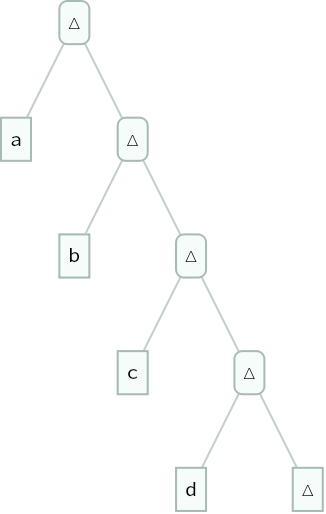
Tree Calculus supports a simple structure for lists
In[]:=
cList[{h_,r__}]:=Node[h,cList[{r}]]
In[]:=
cList[{h_}]:=Node[h,Node]
In[]:=
cList[{a,b,c,d}]//ExpressionTree
Out[]=
As well as a native form of binary trees
Complex Functions
Complex Functions
A program which adds two natural numbers:
The above functions have the expected functionality; size returns the size of any given program (including itself), equality tests for the completely equality of two given programs, and the final tree replicates the behavior of the lambda operator.
Additional Tools
Additional Tools
TreeToFunction converts a tree object into a Tree Calculus program in functional form.
MinimalTreeProg[criteria, size, iterations] checks all possible trees up to size and finds the smallest program that meets a specified criteria after reducing the program up to iterations times.
Here, we search for the smallest version of Not:
The resource function MultiwayCombinator can be used to track the differences in state based on execution priority (ex. root first vs. branch first)