Perimeter of Bernoulli Lemniscate by Two Different Methods
Authors: Housam Binous and Ahmed Bellagi
Perimeter of Bernoulli Lemniscate by Two Different Methods
Authors: Housam Binous and Ahmed Bellagi
Authors: Housam Binous and Ahmed Bellagi
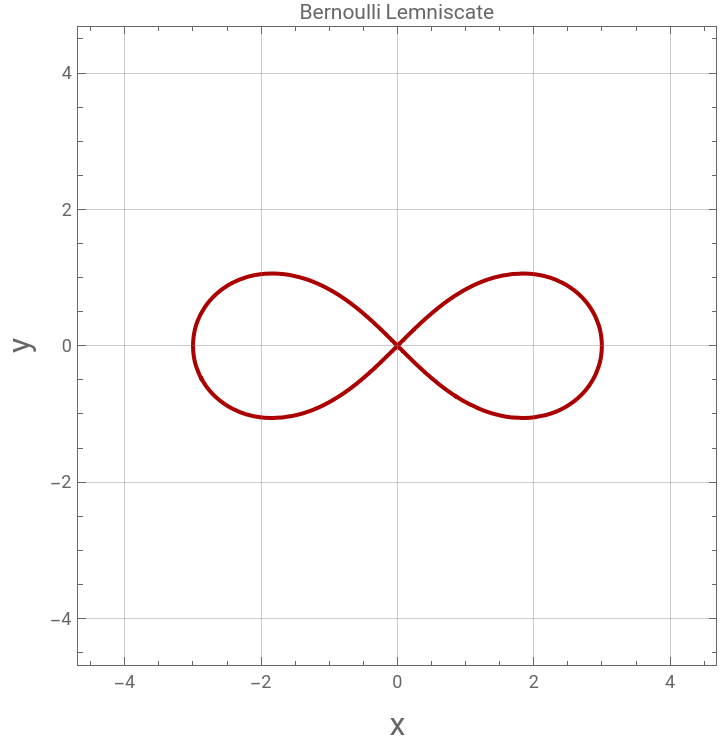
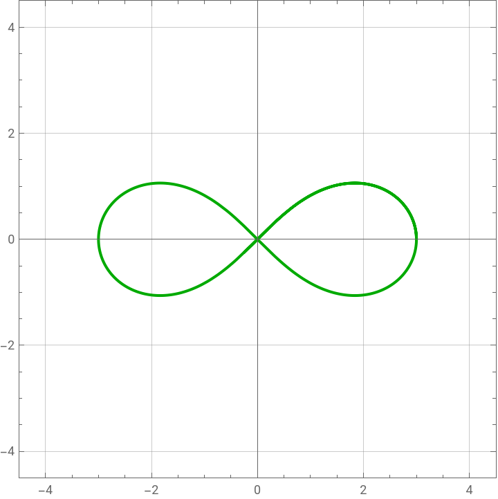
We compute the perimeter of Bernoulli Lemniscate using two different approaches: (1) Elliptic integral formulation and (2) Arc-length continuation (numerical differential approach).The Bernoulli Lemniscate is defined by: =-Method 1: Based on Elliptic IntegralThe exact perimeter of a Lemniscate is given by: where: K(m) is the complete elliptic integral of the first kind.Method 2: Arc-Length Continuation MethodThe second approach is based on the definition of arc length, where the perimeter is computed as the total length of a parametric curve.For , both calculations yield
2
+
2
x
2
y
2
a
2
x
2
y
P=2
2
aK1
2
a=3
P=15.7323
Method based on elliptic integral
In[]:=
a=3.;
In[]:=
p=ContourPlot[(x^2+y^2)^2==a^2(x^2-y^2),{x,-1.5a,1.5a},{y,-1.5a,1.5a},PlotLabel->"Bernoulli Lemniscate",GridLines->Automatic,ContourStyle->{Thick,Darker@Red},AspectRatio->1,FrameLabel->{Style["x",16],Style["y",16]}]
Out[]=
In[]:=
Ltotal_exact=2aSqrt[2]EllipticK[1/2]
Out[]=
15.7323
Method based on arc - length continuation
In[]:=
eq1=(x[s]^2+y[s]^2)^2==a^2(x[s]^2-y[s]^2)(*equationofanellipse*)
Out[]=
2
(+)
2
x[s]
2
y[s]
2
x[s]
2
y[s]
In[]:=
eq2=x'[s]^2+y'[s]^2==1(*auxiliaryequation*)
Out[]=
2
′
x
2
′
y
In[]:=
SOL=Quiet@First@NDSolve[{eq1,eq2,x[0]==a,y[0]==0,x'[0]==0.01,y'[0]==0.01},{x,y},{s,0,20},AccuracyGoal->10]
Out[]=
xInterpolatingFunction,yInterpolatingFunction


In[]:=
ParametricPlot[{x[s],y[s]}/.SOL,{s,0,20},Frame->True,PlotRange->{{-1.5a,1.5a},{-1.5a,1.5a}},GridLines->Automatic,PlotStyle->Darker@Green,ImageSize->Medium,AspectRatio->1]
Out[]=
In[]:=
P=s/.FindRoot[(x[s]/.SOL)==a,{s,20}]
Out[]=
15.7323