ABSTRACT (original article): Analytical techniques for the detection of aldehydes often involve reaction with either a hydrazine or hydroxylamine derivative,resulting in the formation of a hydrazone or oxime, respectively. While there are various examples for the use of either type of derivatization reagent, there have been only few reports with data suitable to answer which of the two types of probes allows faster and more selective detection of aldehydes. Addressing this question, this work used H NMR spectroscopy to study the kinetics of the reactions of aromatic and aliphatic aldehydes with two derivatization probes, phenylhydrazine or O-phenylhydroxylamine, in tetrahydrofuran and in presence of an excess of acid catalyst. A fitting procedure was developed to determine the rate constants of these second order reactions while avoiding use of either aldehyde or probe in a large excess. Hydrazone formation was found to be on average 71 times faster than oxime formation. The rate constants for the reaction of aromatic aldehydes with the phenylhydrazine follow largely the trend predicted by Hammett substituent constants, with the notable exception of the hydrogen bond forming 2-hydroxybenzaldehyde. Unlike in studies with water as solvent, aliphatic aldehydes were not found to react faster than aromatic ones. CITATION (original article): Blair K. Troudt, John W. Vue, Philippe Bühlmann, Comparison of the kinetics of aldehyde sensing by covalent bond formation with hydrazines and hydroxylamines, Tetrahedron, 119, 2022, 132852. https://doi.org/10.1016/j.tet.2022.132852
1
Variables: Ald, Hydr, Product
AldTotal Ald[t] + Prod[t]
HydrTotal Hydr[t] + Prod[t]
Ald'[t] -kzero Ald[t] Hydr[t]
Hydr'[t] -kzero Ald[t] Hydr[t]
Prod'[t] kzero Ald[t] Hydr[t]
Ald[t=0] AldTotal
Hydr[t=0] HydrTotal
Product[t=0] 0
AldTotal Ald[t] + Prod[t]
HydrTotal Hydr[t] + Prod[t]
Ald'[t] -kzero Ald[t] Hydr[t]
Hydr'[t] -kzero Ald[t] Hydr[t]
Prod'[t] kzero Ald[t] Hydr[t]
Ald[t=0] AldTotal
Hydr[t=0] HydrTotal
Product[t=0] 0
The following shows that Mathematica can solve the set of 3 differential equations if no boundary conditions are used. If boundary conditions are included, Mathematica fails to find a solution.
In[]:=
DSolve[{Ald'[t]-kzeroAld[t]Hydr[t],Hydr'[t]-kzeroAld[t]Hydr[t],Prod'[t]kzeroAld[t]Hydr[t]},{Ald[t],Hydr[t],Prod[t]},t]
Out[]=
Hydr[t]C[1]-C[1],Ald[t]-C[1],Prod[t]-C[1]-+C[3]
C[1]C[2]
-+
kzerotC[1]
C[1]C[2]
C[1]C[2]
-+
kzerotC[1]
C[1]C[2]
C[1]C[2]
kzerotC[1]
C[1]C[2]
Here an example with benzaldehyde data:
In[]:=
databenz={{0.`,0.017445`},{0.`,0.017662`},{0.`,0.0177`},{0.`,0.017115`},{361.`,0.0108`},{361.`,0.01005`},{361.`,0.0098778`},{659.`,0.006457`},{659.`,0.006532`},{659.`,0.00775`},{944.`,0.0045`},{944.`,0.0047599999999999995`},{944.`,0.005860000000000001`},{1241.`,0.00385`},{1241.`,0.004`},{1241.`,0.0039`},{1528.`,0.0035`},{1528.`,0.0032`},{1528.`,0.0044`},{1825.`,0.0030800000000000003`},{1825.`,0.0030499999999999998`},{1825.`,0.0039`}}
Out[]=
{{0.,0.017445},{0.,0.017662},{0.,0.0177},{0.,0.017115},{361.,0.0108},{361.,0.01005},{361.,0.0098778},{659.,0.006457},{659.,0.006532},{659.,0.00775},{944.,0.0045},{944.,0.00476},{944.,0.00586},{1241.,0.00385},{1241.,0.004},{1241.,0.0039},{1528.,0.0035},{1528.,0.0032},{1528.,0.0044},{1825.,0.00308},{1825.,0.00305},{1825.,0.0039}}
In[]:=
ListPlot[databenz]
Out[]=
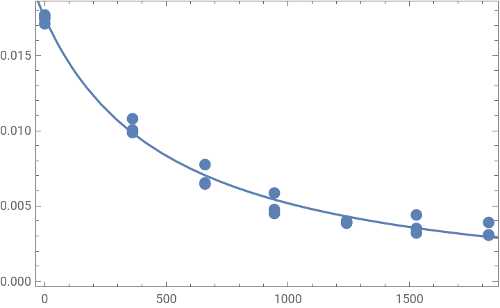
First I just try to fit the benzaldehyde data only using the result of the above solution of the differential equations. The only new trick that is applied is that in the solution the C[1] and C[2] terms are replaced with ‘a’ and ‘b’. Without that replacement, the fit does not work.
In[]:=
FindFitdatabenz,-C[1]/.{C[1]a,C[2]b},{a,b,kzero},t
C[1]C[2]
-+
kzerotC[1]
C[1]C[2]
Out[]=
{a-8.06463,b5.42032,kzero-9.34938}
One could plot the above solution, but the result is an absolutely horrible fit---not even close. This fit will only work if one uses some semi-decent starting values.
To find a good set of starting values for FindFit, the above general solutions for the hydrazine, aldehyde and product are evaluated first at time zero....
In[]:=
Hydr[t]C[1]-C[1],Ald[t]-C[1],Prod[t]-C[1]-+C[3]/.t0
C[1]C[2]
-+
kzerotC[1]
C[1]C[2]
C[1]C[2]
-+
kzerotC[1]
C[1]C[2]
C[1]C[2]
kzerotC[1]
C[1]C[2]
Out[]=
Hydr[0]C[1]-C[1],Ald[0]-C[1],Prod[0]-C[1]+C[3]
C[1]C[2]
-1+
C[1]C[2]
C[1]C[2]
-1+
C[1]C[2]
C[1]C[2]
1-
C[1]C[2]
... and then Hydr[0] and Ald[0] are replaced with the respective total concentrations that are known from the experiment, and Prod[0] is replaced with zero.
In[]:=
SolveHydrtot==C[1]-C[1],Aldtot==-C[1],Prodtot==-C[1]+C[3]/.{Aldtot0.026,Hydrtot0.025,Prodtot0}
C[1]C[2]
-1+
C[1]C[2]
C[1]C[2]
-1+
C[1]C[2]
C[1]C[2]
1-
C[1]C[2]
Out[]=
{{C[1]-0.001,C[2]-39.2207,C[3]0.026}}
Now that good estimates of C[1] and C[2] are available, and one can go back to do the FindFit, but this time with first guesses for ‘a’ and ‘b’ that are much closer. That now gives a much better fit. Note that for Kzero no first guess was needed.
In[]:=
FindFitdatabenz,-C[1]/.{C[1]a,C[2]b},{{a,-0.001`},{b,-39.22071315328157`},kzero},t
C[1]C[2]
-+
kzerotC[1]
C[1]C[2]
Out[]=
{a0.00300461,b-52.6555,kzero0.0996872}
In[]:=
ShowListPlot[databenz,PlotStylePointSize[0.025]],Plot-C[1]/.{C[1]a,C[2]b}/.{a0.0030046123885702275`,b-52.65548371087529`,kzero0.0996872139550311`},{t,-500,2500},FrameTrue
C[1]C[2]
-+
kzerotC[1]
C[1]C[2]
Out[]=
Now the same for the hydrazine data.
In[]:=
dataph={{0.`,0.0228`},{0.`,0.02205`},{0.`,0.0233`},{361.`,0.01158`},{361.`,0.0119`},{659.`,0.0075899999999999995`},{659.`,0.0085`},{944.`,0.005679999999999999`},{944.`,0.0064`},{1241.`,0.00479`},{1241.`,0.00532`},{1528.`,0.0038799999999999998`},{1528.`,0.00441`},{1825.`,0.0031349999999999998`},{1825.`,0.0034500000000000004`}}
Out[]=
{{0.,0.0228},{0.,0.02205},{0.,0.0233},{361.,0.01158},{361.,0.0119},{659.,0.00759},{659.,0.0085},{944.,0.00568},{944.,0.0064},{1241.,0.00479},{1241.,0.00532},{1528.,0.00388},{1528.,0.00441},{1825.,0.003135},{1825.,0.00345}}
In[]:=
ListPlot[dataph]
Out[]=
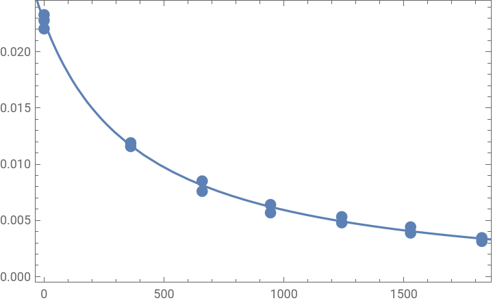
The same guesses for a and b can be used as above, as those had nothing to do with the experimental kinetics data but were only based on the estimated guesses of the starting concentrations. One must plug in the above solution for the hydrazine from the solution of the differential equations.
In[]:=
FindFitdataph,C[1]-C[1]/.{C[1]a,C[2]b},{{a,-0.001`},{b,-39.22071315328157`},kzero},t
C[1]C[2]
-+
kzerotC[1]
C[1]C[2]
Out[]=
{a-0.00230164,b-41.9206,kzero0.100806}
In[]:=
ShowListPlot[dataph,PlotStylePointSize[0.025]],PlotC[1]-C[1]/.{C[1]a,C[2]b}/.{a-0.0023016418304428635`,b-41.92057350977152`,kzero0.1008061929499884`},{t,-500,2500},FrameTrue
C[1]C[2]
-+
kzerotC[1]
C[1]C[2]
Out[]=
Finally, the same for the product.
In[]:=
dataprod={{0.`,0.`},{361.`,0.01024`},{361.`,0.0114`},{361.`,0.0108`},{659.`,0.015269999999999999`},{659.`,0.01494`},{659`,0.01525`},{944.`,0.016980000000000002`},{944.`,0.01753`},{944.`,0.01767`},{1241.`,0.019875`},{1241.`,0.018855`},{1241.`,0.019125`},{1528.`,0.019364999999999997`},{1528.`,0.02028`},{1528.`,0.020114999999999997`},{1825.`,0.021`},{1825.`,0.0197`},{1825.`,0.021`}}
Out[]=
{{0.,0.},{361.,0.01024},{361.,0.0114},{361.,0.0108},{659.,0.01527},{659.,0.01494},{659.,0.01525},{944.,0.01698},{944.,0.01753},{944.,0.01767},{1241.,0.019875},{1241.,0.018855},{1241.,0.019125},{1528.,0.019365},{1528.,0.02028},{1528.,0.020115},{1825.,0.021},{1825.,0.0197},{1825.,0.021}}
In[]:=
ListPlot[dataprod]
Out[]=
One can use the same guesses for ‘a’ and ‘b’ as above, as those had nothing to do with the experimental kinetics data but were only based on the estimated guesses of the starting concentrations. There is one BIG difference, though; in the solution of the differential equation, the product term is the only term that also contains C[3]. However, a good starting value for C[3] is already available from the above evaluation using the estimated starting concentrations of the hydrazine and the aldehyde. One must plug in the above solution for the product from the solution of the differential equations.
In[]:=
FindFitdataprod,-C[1]-+C[3]/.{C[1]a,C[2]b,C[3]c},{{a,-0.001`},{b,-39.22071315328157`},{c,0.026`},kzero},t
C[1]C[2]
kzerotC[1]
C[1]C[2]
This fit looks poor, so I rather also make a starting value guess for kzero.
This is a great fit, but the kzero value is very different from the kzero values of the other fits. It appears that with four fitting parameters, there is just too much freedom. This is confirmed by the following fit and plot, in which kzero is set to a value as it was obtained from the two prior fits, and a, b, and c are fitted. It shows that for a completely different kzero, a good fit is still obtained.
The above highlights a problem that may have already been apparent above, which is that it makes no sense to use different values for ‘a’ and ‘b’ for the aldehyde and hydrazine data; in the same manner, it makes no sense to use different values for ‘a’ and ‘b’ for the aldehyde, hydrazine, and product data.
What should be done is use the Kronecker delta and fit all data in one run.
What should be done is use the Kronecker delta and fit all data in one run.
This can be done by re-listing the data:
This now gives the full dataset, with an initial counter for each data value that identifies the relevant dataset
Let us see how good the plots look like
And just for curiosity, how would this look like if one were to only use the benzaldehyde and hydrazine data?
The only disadvantage of FindFit is that it does not provide confidence intervals. Unfortunately, one cannot use the NonlinearModelFit in this problem. To address this, a Jacknife method may be used.
The following selects a random element from the FullDataSet.
The following gives a random selection of data points from the FullDataSet, where the number of data points in that random selection is half of the number of data points in the full dataset
The following makes a fit to this RandomSelection:
And now all in one step. If that step is evaluated multiple times, one will find that often there is a very similar value for kzero, but once in a while there is a very poor value and the method does not converge.
This is how the kzero from one fit can be selected.
The following gives a list of kzero values obtained from 100 random selections of 80 data points each from the total data.
Values where the fit did not converge can be easily recognized as being negative, so those values can be removed. Using Select[...,#>0&] does that. This shows that on average about 80% of the fits converge.
The following shows the mean of those 87 fits. The mean of kzero is very close to the value obtained from the fit of the full data set, which was 0.128
One can play with the above and make repeated random selections of 100 subsets and make the fits. This was done here, and it seems that the mean is always the same within 1% or 2%. The standard deviation is also always very similar. The following plot shows that the distribution is also fairly symmetrical, so calculating the standard deviation is a reasonable thing to do.
One last issue to look at. How much does the size of the selection for the fit affect the standard deviation? Note that on the x axis is the number of data points in the random selection. Note that each data point is randomly selected from the full data set, so one point may be selected multiple times, and the total number of data points in this random selection may be larger than the number of data points in the original full data set.
Once more the same; this time each random sample contains between 80 and 100 data points, but the standard deviation is calculated in each case from 500 random samples.
I recommend that the standard deviation is estimated from 1000 random samples that each correspond to 80% of the full data set, and round to one digit. So here the standard deviation is 0.006
CITE THIS NOTEBOOK
CITE THIS NOTEBOOK
Nonlinear fitting of reaction kinetics data with Kronecker delta and bootstrapping for uncertainty determination
by Philippe Buhlmann
Wolfram Community, STAFF PICKS, June 20, 2024
https://community.wolfram.com/groups/-/m/t/3197254
by Philippe Buhlmann
Wolfram Community, STAFF PICKS, June 20, 2024
https://community.wolfram.com/groups/-/m/t/3197254