Part 2 of 5—a hydraulic test rig in Saarbrücken, Germany
Real world systems consist of many components. How do you ensure that these components are in a healthy state? When I worked in the oil industry, we had various routines: weekly, monthly, quarterly checks for vibration, pressure and temperature. We had to judge the condition manually, but it was hard and prone to errors. It takes a lot of experience to judge when things are not normal, and by the time we did see that something was wrong, we had already lost days.
So: how can we predict faults early? And since we cannot measure everything, how do we know which component might be faulty? One way is a digital twin: a physics model, synced with sensor data, that tracks the equipment.
In this article, we take a real hydraulic system, build its physics model from its published schematic and calibrate it on its measurements. Then we use the twin to track the system's condition, and predict its future state.
1. The case study
1. The case study
ZeMA, an engineering research centre in Saarbrücken, Germany, built a hydraulic test rig. The researchers ran 2205 working cycles of 60 s each, 36.75 hours in total, and published all the sensor data. You can find it here: https://doi.org/10.24432/C5CW21
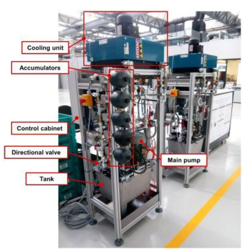
The test rig. Photo from Schneider, Helwig, Klein, Schütze, Proceedings 2(13), 781 (2018), CC BY 4.0.
The rig repeats a 60-second work cycle: In each cycle, the load valve steps the pressure through five levels, and a switching valve opens and shuts. The researchers changed the condition of four components during operation and labelled the corresponding cycle with what they had done. Here are the changes they tested:
◼
Cooler: Efficiency was reduced to 20 %, or nearly off at 3 %. The oil then runs at 36, 45 or 55 °C.
◼
Valve: the switching valve opens on time, with a small lag, a severe lag, or close to failure.
◼
Pump: no internal leakage, weak leakage or severe leakage, emulated with small bypass orifices.
◼
Accumulator: its gas precharge at 130 bar, or lost down to 115, 100 or 90 bar.
So we can build a digital twin and then check it: for every cycle, the labelled data tells what was really wrong so we can validate the response.
Here is the data from three sensors for cooler efficiency, valve opening percentage, leakage through pumps and accumulator pressure.
In[]:=
SetDirectory[NotebookDirectory[]];Get["assets/realrig/ReadRig.wl"];d=RigData["data/hydraulic_zema"];
ConditionsFigure[d]
Out[]=
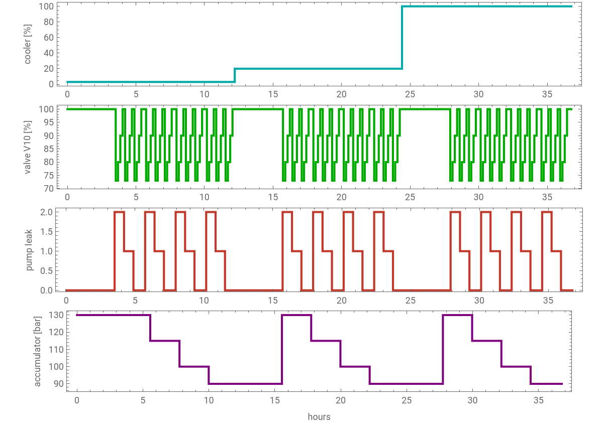
The cooler ran nearly off (3 %) for the first 12 hours, then at 20 %, then at full efficiency. Within each cooler setting, the accumulator lost pressure in steps from 130 to 90 bar, the pump leak was switched on in blocks (0 none, 1 weak, 2 severe), and the switching valve V10 cycled through all four conditions.
2. How the system works
2. How the system works
The hydraulic rig has two circuits that share one 40 L oil tank.
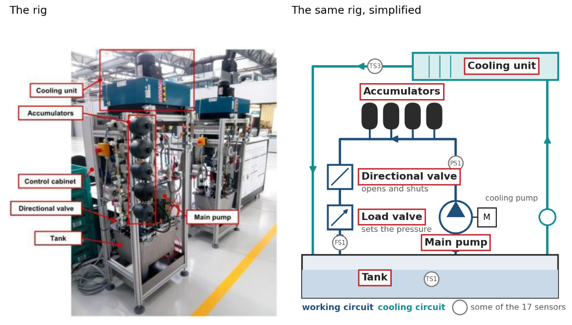
Left: the test rig. Right: the same rig, simplified: the working circuit (blue) and the cooling circuit (teal).
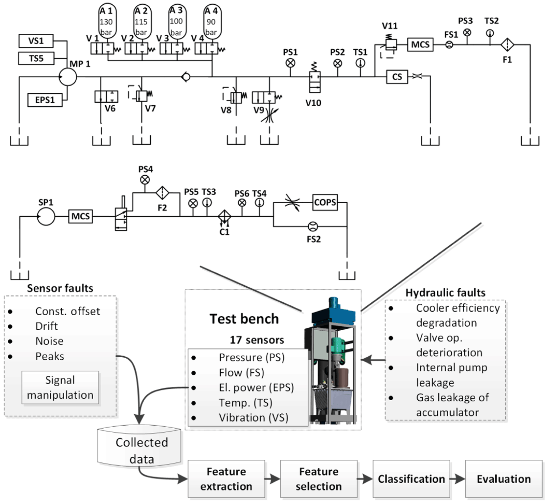
Schematic of the rig. Fig. 2 of Schütze, Helwig, Schneider, J. Sens. Sens. Syst. 7, 359 (2018), CC BY 4.0.
◼
The working circuit (top):
◼
the main pump MP1 pushes about 8 l/min through a check valve.
◼
Four accumulators A1-A4, one switched ON at a time. T
◼
he relief valve V8 caps the pressure at 190 bar, and
◼
the bypass V9 emulates the pump leak.
◼
Then the switching valve V10,
◼
and the load:
◼
a proportional relief valve V11,
◼
followed by the flow meter FS1 and a return filter.
◼
The cooling-filtration circuit (bottom):
◼
a second pump SP1 sends oil through an air-oil cooler and
◼
back to the tank.
In every cycle, V10 shuts for the first 9.5 s, and the pressure climbs to the relief valve's 190 bar. Then V10 opens and the load valve V11 steps the load through five states, resulting in operational pressures from 147 to 167 bar. Here is one cycle, from the data:
In[]:=
dir=CreateDirectory[];zip=URLDownload["https://archive.ics.uci.edu/static/public/447/condition+monitoring+of+hydraulic+systems.zip",dir];(*80MBdownload*)ExtractArchive[zip,dir];read[name_]:=Import[FileNameJoin[{dir,name<>".txt"}],"Table"];{ps1,fs1,eps1}=read/@{"PS1","FS1","EPS1"};
cycle=1790;GraphicsColumnListLinePlotps1[[cycle]],,ListLinePlotfs1[[cycle]],,ListLinePloteps1[[cycle]],
Out[]=
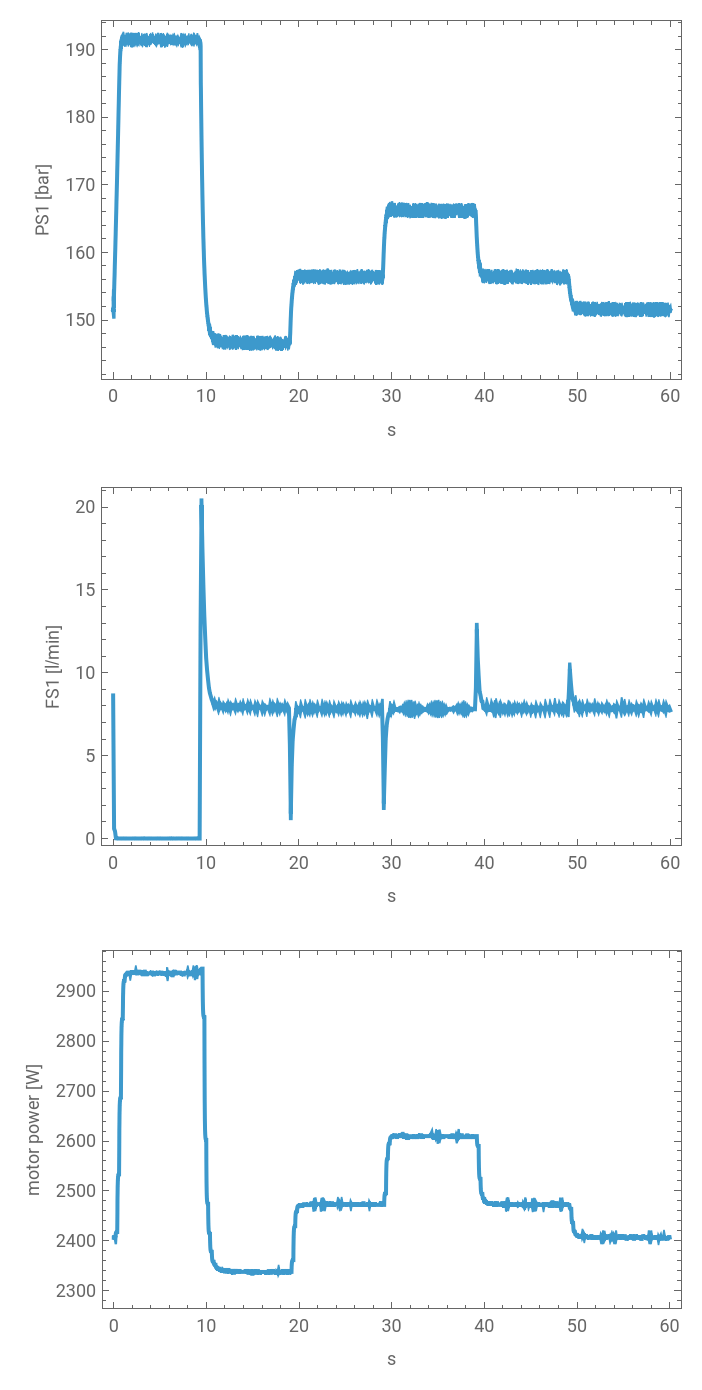
Data: UCI Machine Learning Repository, dataset 447, Helwig, Pignanelli, Schütze (ZeMA), CC BY 4.0.
3. Checking cycles with fault
3. Checking cycles with fault
Here are some faults that have been introduced by the researchers:
◼
Pump leak: the pump delivers less, by 0.22 l/min (weak) or 0.33 l/min (severe). That is 3 to 4 % of its flow.
◼
Valve: V10 opens late, by up to 0.3 s, so the pressure falls later.
◼
Accumulator: with less gas in the accumulator the pressure climbs faster when V10 shuts.
◼
Cooler: the oil runs hotter. Hot oil is thinner and slips past the pump’s gears, so a healthy pump in hot oil delivers less too. On a flow meter, hot oil may look like a faulty pump, and from manual observations the two are very hard to distinguish.
4. The physics model
4. The physics model
I built the model of the rig in Wolfram System Modeler, with version 3.0 of the Hydraulic library, (which will be released soon). It follows the schematic component by component: the pump with its motor, the check valve, the four accumulators behind their switching valves, the relief valves, the leak orifices, V10, the load valve V11, the flow meter, the return filter and the tank.
Because the model is acausal, we don’t just calculate output variables; a change in the downstream load valve (V11) or a fluid temperature spike automatically propagates upstream through the entire network, mirroring the physical rig’s behavior.
The oil is HLP 32. The accumulators are 0.6 L diaphragm units. The leak orifices are 0.2 and 0.25 mm. These come from the rig's description in Helwig's thesis (Saarland University, 2018).
The above circuit is half of the rig. The other half is the cooling-filtration circuit that controls the oil temperature.
The model contains:
◼
the 40 L tank, as two zones: the return side, where the hot oil comes back, and the suction side, where the pumps draw from;
◼
the cooling pump SP1, the air-oil cooler C1 with its fan, and the branch back to the tank;
◼
the steel of the tank and pumps, which stores heat;
◼
the heat lost to the room.
Its input is the heat the working circuit puts into the oil. It gives the oil temperatures TS1, TS3 and TS4, and the cooling flow and pressures, which the rig also measures. This is the model that later forecasts the oil temperature.
5. Calibration
5. Calibration
As in any model, the next step is calibration: I started with searching the values from the literature, then calibrated on the measurements.
◼
The relief valves, V10 and the load valve V11 are tuned from the rig's pressures.
◼
The return line splits into a filter and its fittings. The pressure upstream of the filter scales with viscosity, indicating that the majority of the pressure drop is driven by localized losses in the plumbing fittings.
◼
The pump's slip, the motor's slight slowdown under load, and the leak orifices come from the flow speeds and the motor power.
One result I like: the accumulators' gas volume was left free in the fit, and the data put it at 0.601 l. The datasheet mentioned 0.6 l.
Here you can see the calibrated model against the measured cycles, at 36 °C and 55 °C oil, for all three leak levels:
Thin lines: measured (UCI dataset 447). Dashed: the System Modeler model.
Across all 1216 stable cycles the model tracks the rig to 0.3 bar in pressure, 20 ml/min in flow and 6 W in motor power.
Note on residual deviations: the model tracks most of the cycle closely, but a leaking pump draws 10 W to 45 W more motor power than the bypass orifices account for, more in cold oil than in hot. The pump's viscous friction is already in the model, and it does not change when a bypass opens, so the cause is not known yet; it may be in how the rig emulates the leak. In a production twin, this would be the next thing to model.
6. Calibrated twin
6. Calibrated twin
Once we have a calibrated physics model of the rig, it is time to create a digital twin.
In the first part of the digital twin series, we defined it as a physics model, synced with sensor data, that tracks the equipment. The hydraulic physics model can tell us how a healthy rig would behave, but not how this rig is behaving right now. It becomes a twin when it is kept in sync with data from a real machine.
In this case the twin has three parts:
◼
The model: the calibrated working circuit and the thermal model from the previous sections.
◼
The sync: every 60 s cycle, the model is put in the same state as the rig. It runs the same input signals at rig’s current oil temperature.
◼
The tracking: the twin compares what the sensors measured with what a healthy rig would show in that same state.
Here is a schematics of the process:
The sensors are compared with what the model expects, and the result is checked against the labelled data.
◼
For this twin, the physics model is not running all the time. Before deployment, it was run a few hundred times to learn what each component’s faults look like at every oil temperature; the twin stores those results and compares every cycle with them.
◼
The forecast is different: it is a real simulation of the thermal model, started from the state of the rig at that cycle. For the live page, I ran these simulations for the whole recording beforehand and stored them, so the page only replays them. On a running machine, one forecast takes about a second, so the twin could compute it as each cycle arrives.
Now the question that matters: from the sensors alone, can the twin tell which component is not behaving normally?
The twin runs the same 60-second inputs received during a cycle: when V10 is open or closed, the inputs of V11, and the motor readings. It then predicts and compares the response with the sensor readings and tries to infer the state of the system.
Pump: is it leaking?
Pump: is it leaking?
Let's start with the pump leak. To identify the leak, a twin needs to know what are the typical values of a healthy pump for a given oil temperature. If there is deviation, then it might suggest leak somewhere. The physical model was used to obtain these typical values.
LeakFigure[d, twin, ok]
Here is the same flow reading done two ways. On the left, a person compares the flow with what a healthy pump gave in cool oil, a fixed number from the commissioning sheet. On the right, the twin compares it with what the model says a healthy pump gives at this cycle’s oil temperature.
The person gets 81 % right and calls 146 healthy pumps leaking, every one of them in hot oil: thinner oil slips past the gears, so a healthy pump delivers less. The twin reads 1214 of 1216 cycles right, 99.8 %, and never calls a healthy pump leaking.
Valve V10: does it open on time?
Valve V10: does it open on time?
Next, the valve. When the twin receives a V10 close signal, it times the fall of pressure, and asks the model which condition gives that time. It reads the valve right in all 1216 cycles.
ValveFigure[d, reads]
This works because the twin knows when V10 was told to open: it compares the command with the pressure's response.
Accumulator: is it losing gas?
Accumulator: is it losing gas?
The accumulator acts as a pneumatic shock absorber. When fluid enters, it compresses the nitrogen gas volume, cushioning pressure spikes like a spring. As gas bleeds out over time, the remaining smaller volume creates a much stiffer hydraulic response, causing system pressure to spike significantly faster
The twin sees this when V10 shuts at the start of each cycle and the pressure shoots up to 190 bar. With less gas in the accumulator, the pressure climbs faster. So the twin times how long the pressure takes to go from 160 to 185 bar, and compares that time with what the model says it would be for a healthy accumulator (130 bar of gas) and for the three leaky ones (115, 100 and 90 bar).
The differences are small, a few hundredths of a second, so this reading is the weakest: it gets 73 % of the cycles exactly right, and most of the misses are only one step off, 115 read as 130, for example.
AccFigure[d, twin, reads]
Cooler: how well does it remove heat?
Cooler: how well does it remove heat?
The rig measures the oil temperature going into the cooler and coming out of it, and how much oil flows through it. A healthy cooler with its fan at full speed removes about 176 W per degree; at 20 % it removes about 85 W, and nearly off about 53 W. These three numbers come from the thermal model. The twin picks the nearest one, and it is right in every cycle, because the three are far apart.
CoolerFigure[d, twin, reads]
7. Forecasting of oil temperature
7. Forecasting of oil temperature
The twin can also look ahead. The thermal model takes the motor power, the room temperature and the fan setting, and here it tracks the oil temperature over the whole 36.75 hours.
The thermal model (dashed) against the measured temperatures, all 36.75 hours.
The twin can also forecasts the next hour: as things are, and if the cooler failed now.
8. A dashboard, with your favourite LLM
8. A dashboard, with your favourite LLM
Now let's run the twin on the recording as if it were live.
Here is the cycle the page is playing right now, read back from the cloud:
For reference, this is how the data went into the cloud.
You can come up with a design to render things that matter to you like the rig itself, component's condition and so on. Then let your LLM create the page. It fetches the hour it needs from the Wolfram Cloud and plays each cycle in real time, so the values on the schematic change mimicking the actual rig.
The live twin dashboard created with Claude Desktop.
The live twin: https://www.systemsnotcode.com/labs/pumptwin/
(It takes a few seconds to fetch the data after you open the dashboard)
What the page shows:
◼
The rig with sensor readings.
◼
This cycle, live: pressure, flow and motor power, measured and from the model, updated every second.
◼
Component health: one card per component with the twin's reading.
◼
Oil temperature: the last 90 minutes and the next hour, as things are and if the cooler failed now.
◼
Twin log.
Tools used
Tools used
◼
Wolfram System Modeler, with the Hydraulic library 3.0 (pre-release), the rig model.
◼
Wolfram Language: the calibration and forecasts and plotting.
◼
Wolfram Cloud: the replay data behind the live page, one cloud object per hour of the recording.
◼
An LLM (Claude) for the dashboard page: plain HTML and JavaScript.
◼
Data: Condition monitoring of hydraulic systems, UCI Machine Learning Repository, dataset 447, Helwig, Pignanelli, Schütze (ZeMA), CC BY 4.0.
CITE THIS NOTEBOOK
CITE THIS NOTEBOOK
Digital twin: predictive maintenance of a hydraulic system
by Ankit Naik
Wolfram Community, STAFF PICKS, October 2, 2026
https://community.wolfram.com/t/28235
by Ankit Naik
Wolfram Community, STAFF PICKS, October 2, 2026
https://community.wolfram.com/t/28235