The single cosinor method [1,2,3,4] is employed to model the circadian variation in physiological variables. While the 24-hour component usually accounts for the largest proportion of variability in the data, harmonic terms contribute to shape the circadian rhythms. CosinorFit is introduced both for single and multi-component cosinor model fitting of measured physiological variables.
Circadian Rhythms
Circadian Rhythms
Dr. Halberg introduced the word “circadian” in the 1950s to indicate that when organisms are monitored in the absence of external synchronizers (such as the alternation between light and darkness), they keep cycling with a period that is close to but statistically significantly different from 24 hours.
He then showed that most physiological variables such as blood pressure and heart rate are cycling with a period of approximate 24 hours.
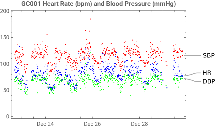
An example of this variation is in a 45 year old female’s measured heart rate and blood pressure measured every 15 minutes day and night over the course of 7 days in TimeSeries GC001:
GC001=TimeSeries[]


Out[]=
Points
Lines
Single Cosinor
Single Cosinor
Now that circadian rhythms have a molecular basis, we learned that the molecular mechanism is conserved across many species over many millennia, a testament to their importance for health and survival.
Dr. Halberg introduced the single and population-mean cosinor models to quantify and compare time structures in health and disease. The single cosinor formula :
Dr. Halberg introduced the single and population-mean cosinor models to quantify and compare time structures in health and disease. The single cosinor formula :
M+Cost+
A
1
2π
τ
1
ϕ
1
(
1
)Applying a 24-hour cosinor model to systolic blood pressure (SBP) measurements in GC001 using :
NonlinearModelFit
In[]:=
c1Model=M+A[1]Cos[t+ϕ[1]];GC001sbp=GC001["PathComponent","SBP"];
2π
τ[1]
In[]:=
timeReference=DateObject@PadRight[DateList[GC001sbp["FirstDate"]][[1;;3]],6];
In[]:=
{times,values}=Transpose[GC001sbp["Path"]];
In[]:=
times0=times-AbsoluteTime@timeReference;
In[]:=
data=Transpose[{times0,values}];
In[]:=
c1Model24=c1Model/.τ[1]QuantityMagnitude[,"Seconds"];
In[]:=
c1NLM=NonlinearModelFit[data,c1Model24,{M,A[1],ϕ[1]},t];
Plotting the fitted model overlaid with the SBP measurements:
Out[]=
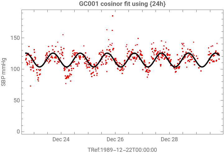
For the most part, the single cosinor model is a “fit”, but it misses the morning and evening peaks and the nighttime drop.
CosinorFit
CosinorFit
CosinorFit
M+Cost++Cost+
A
1
2π
τ
1
ϕ
1
A
2
2π
τ
2
ϕ
2
(
2
)The 2-component cosinor is specified with using the periods of 24h and 12h:
CosinorFit
In[]:=
CosinorFit=ResourceFunction@ResourceObject@"https://wolfr.am/1nLe53Y8Y";(*CosinorFitisintendedtobefinalizedasaWFRinthefuture*)c2Fit=CosinorFit[GC001sbp,{mesor,{,amplitude1,phase1},{,amplitude2,phase2}},{mesor,amplitude1,phase1,amplitude2,phase2},t,timeReference];
Plotting the fitted model overlaid with the SBP measurements:
Out[]=
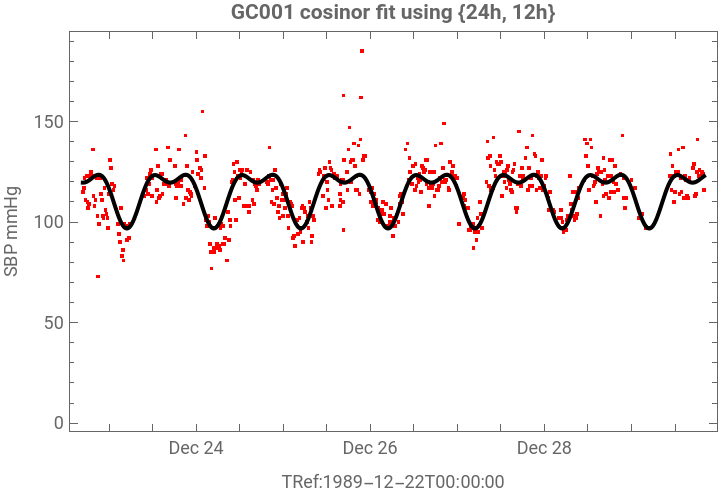
The 2-component cosinor fit approximates the 24-hour changes in the data better than the earlier single component cosinor. A future community post will explore more in detail about the fit metrics and how a Least Squares Spectral Analysis (LSSA) is utilized for non-equidistant data to determine what periodic components contribute most to the variations observed in the data.
Concluding Remarks
Concluding Remarks
The medical profession still relies upon single blood pressure measurements for diagnosis. Use of the cosinor to assess the circadian variation in SBP shows a predictable daily variation of 22.8 mmHg in Systolic blood pressure of a clinically healthy woman over 24 hours. The medical diagnosis should not depend on when during the day the physician takes a measurement of blood pressure. Use of the CosinorFit code for blood pressure and other physiological variables, some of them easily measured with wearable devices should help bring this knowledge to mainstream medicine.
Acknowledgments
Acknowledgments
With appreciation to WSS24 mentors Bob Nachbar, Daniel Sanchez, Daniel Lichtblau and Stephen Wolfram.
References
References
1
.Halberg et al. (1967), “Circadian system phase - an aspect of temporal morphology; procedures and illustrative examples,” In: Proc. International Congress of Anatomists. In: Mayersbach H v, ed. The Cellular Aspects of Biorhythms. Springer-Verlag, New York, 1967; pp. 20-48.
2
.Nelson et al. (1979) Methods for cosinor-rhythmometry. Chronobiologia 6: 305-323.
3
.Bingham et al. (1982), “Inferential statistical methods for estimating and comparing cosinor parameters”, Chronobiologia 9: 397-439.
4
.Cornelissen (2014), “Cosinor-based rhythmometry”, Theoretical Biology and Medical Modelling 2014; 11: 16. 24 pp. https://doi.org/10.1186/1742-4682-11-16
Cite This Notebook
Cite This Notebook
“Implementing cosinor rhythmometry in the Wolfram Languages”
by A. Chase Turner and Germaine Cornélissen
https://community.wolfram.com/groups/-/m/t/3208866
by A. Chase Turner and Germaine Cornélissen
https://community.wolfram.com/groups/-/m/t/3208866