Urban environments, characterized by dense populations and complex ecological systems, present unique results for disease spread. This essay explores epidemiological modeling to understand disease transmission among NYC rats, using both geospatial and network-based graphs. By analyzing rat sighting data, I constructed a geographic plot and a nearest-neighbor graph to represent rat interactions and proximity. Then I simulated disease spread by introducing infected rats and examining its potential impact on the population. This study highlights the application of geographic data and network theory in urban epidemiology, and can be used to see insights into disease dynamics and potential public health interventions.
Introduction
Introduction
New York City, one of the most densely populated urban areas in the world, gives us an opportunity to explore the dynamics of disease transmission inside a highly interconnected urban ecosystem. The city’s high population density is mirrored by a substantial rat population, which is common in the city’s streets, underground tunnels, and subway systems. Rats are the biggest carriers of a range of infectious diseases that pose significant health risks to human populations. Diseases such as leptospirosis, hantavirus, and rat-bite fever are transmitted from rats to humans and can lead to severe health issues. Understanding how these diseases spread through rat populations is crucial for public health efforts aimed at preventing and controlling outbreaks. By using extensive data on rat sightings, we can construct detailed models to represent rat interactions, spatial distributions, and potential disease transmission pathways.
Network Construction
Network Construction
Processing Data from NYC Rat Sightings
Processing Data from NYC Rat Sightings
Importing Data
Importing Data
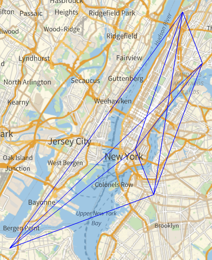
We start with a database of approximately 86,000 rat geolocations, presumably extracted from camera sightings. The dataset utilized includes descriptions of rat sightings reported to the Department of Health and Mental Hygiene in NYC from January 2010 - present (2024).
The following code processes the data by extracting the geographic locations of all reported sightings, then filtering out records where the geo-location is missing or marked as “NotAvailable,” ensuring only valid data is retained.
The following code processes the data by extracting the geographic locations of all reported sightings, then filtering out records where the geo-location is missing or marked as “NotAvailable,” ensuring only valid data is retained.
In[]:=
ratData=Cases[Normal[ResourceData["NYC Rat Sightings"][All,"GeoLocation"]],Except[Missing["NotAvailable"]]];
Finally, we take the clean geocoordinate data of the rats.
In[]:=
ratCoordinates=ratData[[All,1]];
Generate Graph
Generate Graph
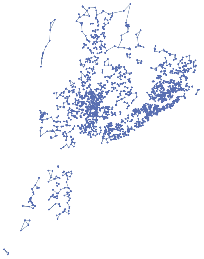
The following function forms a graph of rat sightings based on two parameters:
◼
Amount of sightings
◼
Connectivity distance between rats, defined within a specified geographic range in miles, since rats that are relatively far apart have no chance of infecting each other.
generateRatGraph[numRats_,transmitDistance_]:=NearestNeighborGraph[Take[ratCoordinates,numRats],{All,transmitDistance},DistanceFunction->(QuantityMagnitude[GeoDistance[#1,#2]]&),VertexSize->0.08]Rasterize/@ generateRatGraph[1000,.5]
In[]:=
Select Initial Infection Points
Select Initial Infection Points
This function generates the initial state of the graph based on the infection rate, which denotes the percentage of rats that are initially infected.
However, a rat will only be initialized as infected if it’s connected to at least one other rat. This ensures that only rats that are part of the interaction network are considered for infection, as unconnected rats are insignificant in our simulation.
However, a rat will only be initialized as infected if it’s connected to at least one other rat. This ensures that only rats that are part of the interaction network are considered for infection, as unconnected rats are insignificant in our simulation.
In[]:=
setInfected[infectedRate_,ratGraph_]:=Module[{infectedVertices={}},DeleteDuplicates[Flatten[DeleteCases[If[RandomReal[]<infectedRate && Length[AdjacencyList[ratGraph,Part[VertexList[ratGraph],#]]] != 0 ,AppendTo[infectedVertices,Part[VertexList[ratGraph],#]]]&/@Range[Length[VertexList[ratGraph]]],Null],1]]]
For a infection rate of 3 % and a population of 2500 rats, the starting locations would be
In[]:=
setInfected[0.03,ratGraph]
Out[]=
{{40.8326,-73.8982},{40.7975,-73.9517},{40.848,-73.8497},{40.7609,-73.9577},{40.8181,-73.9285},{40.5791,-73.9834},{40.8296,-73.9204},{40.8293,-73.9189},{40.8829,-73.8836},{40.6802,-73.9454},{40.6554,-73.9301},{40.7765,-73.9451},{40.7195,-73.7445},{40.6725,-73.9104},{40.6728,-73.9071},{40.8066,-73.9407},{40.6353,-73.9633},{40.6711,-73.916},{40.6809,-73.878},{40.8367,-73.9454},{40.6892,-73.9311},{40.6659,-73.8972},{40.744,-73.978},{40.8037,-73.9635},{40.6759,-73.9177},{40.7791,-73.9815},{40.7763,-73.9459},{40.7613,-73.916},{40.7961,-73.9713},{40.6997,-73.9307},{40.7417,-73.8565},{40.6895,-73.9413},{40.7264,-73.9788},{40.777,-73.9456},{40.6759,-73.8736},{40.678,-73.8964},{40.7862,-73.8121},{40.6807,-73.9712},{40.7424,-73.9837},{40.6407,-73.9522},{40.7223,-73.9784},{40.7139,-73.9402},{40.8637,-73.9015},{40.7614,-73.9996},{40.8385,-73.8701},{40.8051,-73.939},{40.8415,-73.8433},{40.7177,-73.941},{40.849,-73.9374},{40.6148,-74.1022},{40.8151,-73.921},{40.7317,-74.001},{40.7188,-73.9957},{40.7592,-73.9324},{40.8533,-73.9076},{40.6685,-73.8094},{40.702,-73.9481},{40.7026,-73.9221},{40.8455,-73.9072},{40.8763,-73.9039},{40.8225,-73.9493},{40.6857,-73.9208},{40.6725,-73.9169},{40.6248,-74.0246},{40.7878,-73.9794},{40.8254,-73.9178},{40.6101,-74.0999},{40.6727,-73.9651},{40.892,-73.8479},{40.7148,-73.9916},{40.819,-73.9405},{40.6889,-73.9594}}
Simulation of Disease Spread
Simulation of Disease Spread
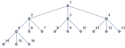
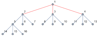
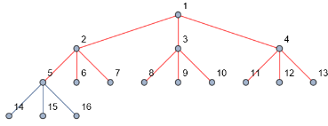
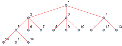
Here is the simulation run on a simple graph, with equal infection spread probabiity, starting from vertex one.
Infection Probability Equation
Infection Probability Equation
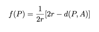
But if we want it to depend on the distance between them, we should calculate the probability that infected rats will transmit disease to other rats through a function of distance between them.
The following function models the likelihood of disease transmission between two rats in a population based on:
The following function models the likelihood of disease transmission between two rats in a population based on:
◼
geographic distance [d(P,A)]
◼
specified interaction radius [r] This equation yields the highest probabilities when rats are at the same location and decreases as the distance between them approaches the interaction radius.
In[]:=
diseaseSpreadProbability[v1_, v2_,radius_]:= 1/(2*radius)*((2*radius)-QuantityMagnitude[GeoDistance[v1,v2]])
For example, we can find the probabiity of two rats who are 12.7107 miles vs two rats who are 3.37626 miles away when their connecting radius is 15 miles.
In[]:=
rat1=vertices[[1]];rat2=vertices[[2]];rat3=vertices[[3]];diseaseSpreadProbability[rat1,rat2,15]diseaseSpreadProbability[rat1,rat3,15]
Out[]=
0.576309
Out[]=
0.887458
Modeling the Expansion
Modeling the Expansion
This function models the spread of a disease through a rat population over a specified number of days. It takes in the
◼
graph of the rat population
◼
a list of initially infected rats
◼
number of days to run the simulation
◼
interaction radius that determines how far apart rats can be for the disease to spread.
The main operation is a loop that iterates through each day of the simulation. For each day, the function evaluates which neighboring rats of the currently infected rats will become newly infected. This evaluation is done by calculating the probability of disease transmission between the infected rat and each of its neighbors based on the distance between them and the interaction radius. If a randomly generated number falls below this probability, the neighbor rat is added to the list of newly infected rats.
After identifying the newly infected rats, the function updates the list of infected rats to include these new additions and visualizes how the infection evolves over time.
In[]:=
infectionSimulate[graph_,infectedRats_,days_,radius_]:= Module[{edges = EdgeList[graph],vertices = VertexList[graph],infected = infectedRats,newInfected={},progressions = {graph}},Do[newInfected = Join[newInfected,Flatten[Pick[AdjacencyList[graph,Part[infected,#]],Thread[Greater[MapThread[diseaseSpreadProbability,{Table[Part[infected,#],Length[AdjacencyList[graph,Part[infected,#]]]],AdjacencyList[graph,Part[infected,#]],Table[radius,Length[AdjacencyList[graph,Part[infected,#]]]]}],RandomReal[]]],True]&/@Range[Length[infected]],1]];infected = Union[infected,newInfected];AppendTo[progressions,Overlay[{HighlightGraph[graph,{Style[infected,Red],Style[Subgraph[graph,infected,EdgeList[Subgraph[graph,infected]]],Red]}],Style["Days: "<>ToString[day],16,Red]}]];,{day,1,days}];infected=Union[infected,newInfected];AppendTo[progressions,Overlay[{HighlightGraph[graph,{Style[infected,Red],Style[Subgraph[graph,infected,EdgeList[Subgraph[graph,infected]]],Red]}],Style["Simulation End",16,Red]}]];AnimatedImage[Rasterize/@progressions,FrameRate->2]]
Factors In Epidemic Modeling
Factors In Epidemic Modeling
This function that starts the simulation, and takes four parameters specified in the previous functions and initiates the entire simulation.
The main factors in order to model a epidemic spread are:
◼
Number of Rats (numRats): Larger populations better represent the variability and complexity of real-world scenarios. So, for the generateSimulation function, a higher number of rats, such as 1,000 or more, is optimal for more realistic simulations.
◼
Interaction Radius (radius): Studies of rat behavior and disease transmission suggest that rats can spread diseases within a few meters. In urban environments, the interaction radius might be around .1 to .3 miles, depending on the type of disease and rat behavior.
◼
Initial Infection Rate (rate): The initial infection rate affects how many rats start out with the disease and can vary from very low to moderate levels. In the spread of the plague in rat populations often starts with 1% to 5% of the population infected. Therefore, setting a rate between 0.01 and 0.05 (1% to 5% of the population) is generally effective for exploring different scenarios of disease introduction and outbreak.
◼
Simulation Duration (days): The duration of the simulation should be long enough to observe the full progression of the disease. For example, a simulation studying the spread of the Ebola virus in animal populations might last for several months. Therefore, setting the number of days to at least 10 and up to 30 days ensures that the simulation covers the disease’s initial spread.
If we were to input "default" parameters
If we were to increase the connection radius.
If we were to increase the amount of nodes.
Finding Optimal Mitigation Points
Finding Optimal Mitigation Points
Optimal mitigation points represent locations where interventions, such as vaccination centers or testing facilities, would have the maximum impact in controlling the disease spread. These points are identified based on their high connectivity and strategic importance within the network of possible disease transmission routes. By focusing on these key locations, public health efforts can efficiently allocate resources to disrupt the transmission chains most effectively.
We first initialize a counter for each vertex to track how often it gets infected. For each day, the infected list is determined by comparing the disease spread probability to a random value for each neighbor of currently infected nodes. The infection status is updated, and the visit count for each infected vertex is incremented and finally, it outputs a list of most checked nodes.
We first initialize a counter for each vertex to track how often it gets infected. For each day, the infected list is determined by comparing the disease spread probability to a random value for each neighbor of currently infected nodes. The infection status is updated, and the visit count for each infected vertex is incremented and finally, it outputs a list of most checked nodes.
By applying the following function using different sectors of NYC, we are able to focus on different highlight areas in order to identify behaviors in the central nodes.
A visual representation of the most checked coordinates in a single simulation. In this specific sector of NYC, coordinate C5 is the most prevalent. (Washington Avenue in the Manhattan Area)
This returns a list of the streets with the most frequent rat interactions with an association to the number of connections it checks through
Conclusion and Future Directions
Conclusion and Future Directions
Conclusion
Conclusion
Through this project, I achieved a comprehensive understanding of how disease spreads among NYC’s rat population using geospatial and network-based modeling techniques. learned how to construct geographic plots and evolving graphs to represent rat interactions accurately. Simulating disease spread by introducing infected rats allowed me to examine the infection’s impact over time, improving my understanding of epidemic dynamics in urban environments.
I improved my skills in processing large datasets, filtering out invalid data, and applying complex functions to model disease transmission probabilities based on geographic distance and interaction radius. The simulation highlighted the importance of factors such as population size, interaction radius, initial infection rate, and simulation duration in accurately modeling epidemic spread. Moreover, I was able to identify optimal mitigation points, such as central hubs in NYC, where interventions would be most effective in controlling disease spread, demonstrating the practical application of this research in public health. This project underscored the value of integrating geographic data and network theory in urban epidemiology, providing critical insights into disease dynamics and potential strategies for preventing and managing outbreaks in densely populated urban areas.
I improved my skills in processing large datasets, filtering out invalid data, and applying complex functions to model disease transmission probabilities based on geographic distance and interaction radius. The simulation highlighted the importance of factors such as population size, interaction radius, initial infection rate, and simulation duration in accurately modeling epidemic spread. Moreover, I was able to identify optimal mitigation points, such as central hubs in NYC, where interventions would be most effective in controlling disease spread, demonstrating the practical application of this research in public health. This project underscored the value of integrating geographic data and network theory in urban epidemiology, providing critical insights into disease dynamics and potential strategies for preventing and managing outbreaks in densely populated urban areas.
Extensions
Extensions
◼
Currently, the model focuses only on rat populations and how diseases spread among them. By adding a component for human locations and interactions, we could simulate how diseases might jump from rats to humans. This could involve mapping out where people live, work, and travel, and then examining how rats and humans might come into contact.
◼
Another way to extend the model is by making it dynamic, with rats and humans moving around. Right now, the positions of rats and humans are fixed, which doesn’t reflect real-life movement. Adding random or pattern-based movement for both rats and humans could make the model more realistic. For example, we could simulate how rats wander through streets or how people commute between different locations.
◼
Expanding the model to study different diseases is another valuable extension. The current model focuses on a single disease with a fixed transmission probability. By introducing various diseases, each with different spread mechanisms, we could explore how different pathogens behave under similar conditions.
Shortcomings
Shortcomings
◼
One major shortcoming of the model is that as the number of rats and the complexity of their interactions increase, the computational requirements grow significantly. This means that larger, more detailed simulations can be slow or even unmanageable with limited resources.
◼
Another limitation is the assumption of uniform behavior among rats. The model assumes that all rats have the same infection probability and interaction radius, which isn’t true in reality. Rats vary in behavior, and their interactions can be influenced by different factors. To make the model more accurate, we could introduce variability in these parameters, such as having different probabilities for different rats or adjusting the interaction radius based on specific conditions.
◼
The current model uses historical data, which may not reflect current conditions or recent changes. Using updated data or adding more diverse data sources could improve the model’s accuracy. For example, incorporating recent sightings or environmental data could help make the model more relevant and precise.
Acknowledgements
Acknowledgements
Thank you to my mentor, William Wei, and TA, Tianyi Gu, for their invaluable support throughout this project. I truly could not have achieved this without their expertise and guidance. I also want to thank the entire team at the WSRP for creating such a supportive and inspiring environment.
References
References
◼
[1] Brooks, D., & Matta, J. (2019, October 26). Spreading of rodent infestations through a city - applied network science. SpringerOpen. https://appliednetsci.springeropen.com/articles/10.1007/s41109-019-0212-6
◼
[2] Gupta, M. (2023, March 6). Rat-bite fever. StatPearls [Internet]. https://www.ncbi.nlm.nih.gov/books/NBK448197/#:~:text=It%20is%20usually%20transmitted%20by,contaminated%20with%20feces%20or%20urine
◼
[3] Rat sightings in NYC. (n.d.-b). https://homepage.divms.uiowa.edu/~luke/STAT4580-samples/rats.html
◼
[4] Rats, cities, people, and pathogens: A systematic review and narrative synthesis of literature regarding the ecology of rat-associated zoonoses in urban centers | vector-borne and Zoonotic Diseases. (n.d.). https://www.liebertpub.com/doi/abs/10.1089/vbz.2012.1195
CITE THIS NOTEBOOK
CITE THIS NOTEBOOK
Epidemiological modeling of disease spread among urban rat populations
by Abhirami Thiagarajan
Wolfram Community, STAFF PICKS, July 12, 2024
https://community.wolfram.com/groups/-/m/t/3216394
by Abhirami Thiagarajan
Wolfram Community, STAFF PICKS, July 12, 2024
https://community.wolfram.com/groups/-/m/t/3216394