ABSTRACT (original article): The global pandemic of COVID-19 over the last 2.5 years have produced an enormous amount of epidemic/public health datasets, which may also be useful for studying the underlying structure of our globally connected world. Here we used the Johns Hopkins University COVID-19 dataset to construct a correlation network of countries/regions and studied its global community structure. Specifically, we selected countries/regions that had at least 100,000 cumulative positive cases from the dataset and generated a 7-day moving average time series of new positive cases reported for each country/region. We then calculated a time series of daily change exponents by taking the day-to-day difference in log of the number of new positive cases. We constructed a correlation network by connecting countries/regions that had positive correlations in their daily change exponent time series using their Pearson correlation coefficient as the edge weight. Applying the modularity maximization method revealed that there were three major communities: (1) Mainly Europe + North America + Southeast Asia that showed similar six-peak patterns during the pandemic, (2) mainly Near/Middle East + Central/South Asia + Central/South America that loosely followed Community 1 but had a notable increase of activities because of the Delta variant and was later impacted significantly by the Omicron variant, and (3) mainly Africa + Central/East Canada + Australia that did not have much activities until a huge spike was caused by the Omicron variant. These three communities were robustly detected under varied settings. Constructing a 3D “phase space” by using the median curves in those three communities for x-y-z coordinates generated an effective summary trajectory of how the global pandemic progressed. CITATION (original article): Hiroki Sayama (2022), Detecting Global Community Structure in a COVID-19 Activity Correlation Network, arXiv:2206.03181. DOI: https://doi.org/10.48550/arXiv.2206.03181
Dataset
Dataset
The dataset used was released by the Center for Systems Science and Engineering (CSSE) at Johns Hopkins University [1,2]. It is time series data of the cumulative numbers of COVID-19 positive cases for 285 countries/regions over the time period from January 22, 2020 to May 29, 2022.
In[]:=
SetDirectory[NotebookDirectory[]];
In[]:=
dataorig=Import["time_series_covid19_confirmed_global-05292022.csv"];
In[]:=
k=3;data={dataorig[[1,Join[Range[4],Range[5+k,Length[dataorig[[1]]]-k]]]]};Do[AppendTo[data,Join[row[[;;4]],Table[Mean[row[[i-k;;i+k]]]//N,{i,5+k,Length[row]-k}]]],{row,dataorig[[2;;]]}];
In[]:=
dates=data[[1,5;;]];
We select only countries/regions that had at least 100,000 cumulative positive cases
In[]:=
data2=Select[data,#[[-1]]>=100000&];data=Prepend[data2,data[[1]]];
In[]:=
newPosCount[i_,date_]:=Module[{dateloc},dateloc=Position[data[[1]],date][[1,1]];Max[data[[i,dateloc]]-data[[i,dateloc-1]],0]];
In[]:=
data[[1,{1,2,3,4,5,-1}]]
Out[]=
{Province/State,Country/Region,Lat,Long,1/25/20,5/26/22}
In[]:=
logpositive[x_]:=If[x<=1,0,Log[x]];
In[]:=
logvecs=Table[Clip[#,{-7,7}]&/@(Table[logpositive[newPosCount[i,d]],{d,dates[[2;;]]}]//Differences)(*addDifferences,clippingwithin+/-7!!*),{i,Range[2,Length[data]]}];
Communities in the global COVID-19 activity correlation network
Communities in the global COVID-19 activity correlation network
Figure 1: Global community structure detected in the COVID-19 activity correlation network using the modularity maximization method [26, 27]. Nodes represent countries/regions that had at least 100,000 cumulative positive cases as of May 29, 2022 in the Johns Hopkins University COVID-19 data repository [1,2]. Edges represent positive correlations of the COVID19 activities in terms of the daily change exponent time series. Three major communities (1, 2, 3) were detected, together with two tiny ones (4, 5) in this example.
(*edgeweights=Flatten[Table[(ij)->(1-CosineDistance[logvecs[[i]],logvecs[[j]]]),{i,Length[logvecs]-1},{j,i+1,Length[logvecs]}]];*)edgeweights=Flatten[Table[(ij)->If[Total[logvecs[[i]]]==0||Total[logvecs[[j]]]==0,0.,Correlation[logvecs[[i]],logvecs[[j]]]],{i,Length[logvecs]-1},{j,i+1,Length[logvecs]}]];nodenames=Table[i->If[#[[2]]!="",#[[1]]<>": "<>#[[2]],#[[1]]]&[data[[i+1,{2,1}]]],{i,Length[logvecs]}];
In[]:=
edgeweights=Select[edgeweights,#[[2]]>0&];
In[]:=
g=Graph[First/@edgeweights,EdgeWeightedgeweights];
In[]:=
comm=FindGraphCommunities[g,Method->"Modularity"]CommunityGraphPlot[g,comm,VertexLabels->nodenames,VertexSize0.5,VertexStyle->Gray,EdgeStyleDirective[LightGray,Opacity[0.2]],VertexLabelStyleDirective[FontSize->12],CommunityRegionStyle"Pastel",CommunityLabels(Style["Community "<>ToString[#],FontSize->14]&/@Range[Length[comm]]),Method->"Hierarchical",ImageSize->1200]
Out[]=
{{2,13,18,24,35,43,48,54,56,65,67,75,80,81,83,85,96,99,100,107,108,109,110,114,117,119,121,122,124,128,132,11,12,23,28,29,39,42,50,58,69,97,116,136,125,115},{1,3,5,14,15,16,19,20,22,34,37,40,44,57,59,63,64,66,68,71,73,77,88,92,95,102,103,106,111,113,118,123,127,130,131,134,135,137,45,76,105},{4,8,10,17,21,27,30,31,32,33,38,41,47,51,62,70,74,82,86,93,98,104,112,126,129,133,139,6,9,49,53,60,79,87,89,91,94,7,72,138},{25,36,120},{61,90}}
Out[]=
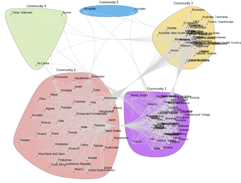
Figure 2: The following are time series plots of the daily change exponents for the three major communities. Thin blue lines show the exponent time series of individual countries (listed on the right), whereas thick blue lines show the median trend curve for each community. When the exponent was positive (negative) the number of daily new positive cases was growing (shrinking). Note that the actual peaks of the COVID-19 activities were where the median trend curve switched its sign from positive to negative, and not where the curve peaked in these plots.
In[]:=
medianline[c_]:=Module[{},Median/@(logvecs[[c]]//Transpose)];
In[]:=
nodenamesdict=<|nodenames|>;
In[]:=
Table[nodenamesdict[c],{c,Complement[Keys[nodenames],VertexList[g]]}]
Out[]=
{Cambodia,Egypt,France: Martinique,Georgia,Kyrgyzstan,Luxembourg,Oman}
In[]:=
Quiet[datesforplotting=DateObject/@dates[[3;;]]];Do[Show[DateListPlot[{datesforplotting,medianline[comm[[i]]]}//Transpose,PlotRange->All,PlotStyle->Directive[Thick,Blue],Joined->True,FrameLabel->{"Date","Daily change exponent"},PlotLabel->"Community "<>ToString[i],LabelStyle->Black,ImageSize->450],DateListPlot[({datesforplotting,#}//Transpose)&/@logvecs[[comm[[i]]]],Joined->True,PlotRange->{Min[#]-0.01,Max[#]+0.01}&[medianline[comm[[i]]]],PlotStyle->Directive[Blue,Opacity[0.01]],PlotLabel->"Cluster "<>ToString[i],PlotLegendsTable[nodenamesdict[c],{c,comm[[i]]}]]]//Print,{i,Length[comm]}]
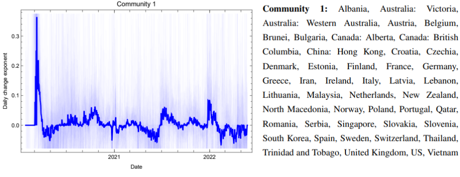
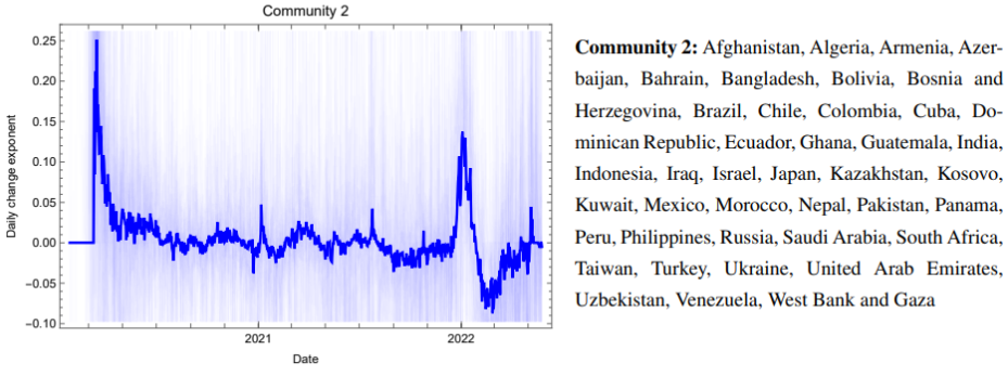
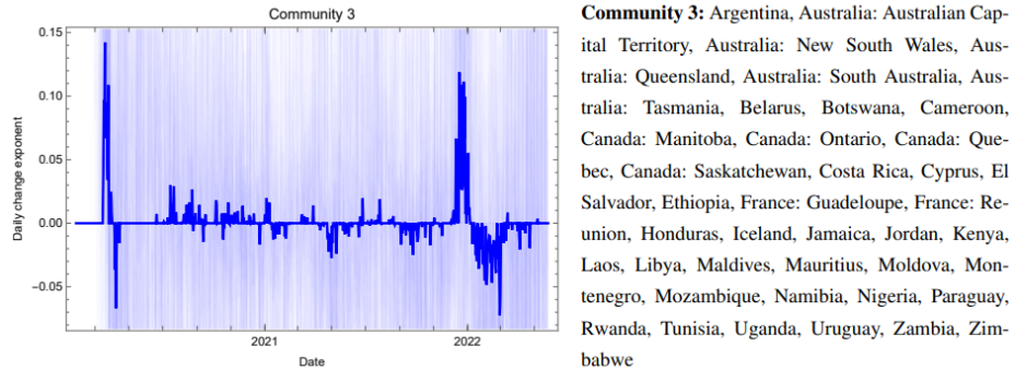
The following is Three-dimensional “phase space” visualization of the global pandemic state. The trajectory was constructed using the median trend curves of the daily change exponents for the three major communities (Communities 1, 2, and 3 as shown in Figure 2) for x, y, and z coordinates, respectively. The trajectory was smoothed using the B-spline algorithm for visualization purposes. Arrowheads indicate the direction of time.
(a) Trajectory for the entire period of collected data.
(b) Initial outbreak in January–April 2020, in which the activities spread in a sequence from Community 1 to Community 2, and then to Community 3.
(c) Outbreak of the Omicron variant in December 2021 and January 2022, in which the activities spread in a different direction from Community 3 to Communities 1 and 2.
References
References
◼
1. Dong, E., Du, H., & Gardner, L. (2020). An interactive web-based dashboard to track COVID-19 in real time. The Lancet Infectious Diseases, 20(5), 533–534.
◼
2. Center for Systems Science and Engineering (CSSE) at Johns Hopkins University. COVID19 Data Repository. https://github.com/CSSEGISandData/COVID-19. Accessed on June 5, 2022.
◼
26. Blondel, V. D., Guillaume, J. L., Lambiotte, R., & Lefebvre, E. (2008). Fast unfolding of communities in large networks. Journal of Statistical Mechanics: Theory and Experiment, 2008(10), P10008.
◼
27. Wolfram Language & System Documentation. FindGraphCommunities. https://reference.wolfram.com/language/ref/FindGraphCommunities.html. Accessed on June 5, 2022.
CITE THIS NOTEBOOK
CITE THIS NOTEBOOK
Detecting Global Community Structure in a COVID-19 Activity Correlation Network
by Hiroki Sayama
Wolfram Community, STAFF PICKS, October 26, 2023
https://community.wolfram.com/groups/-/m/t/3056172
by Hiroki Sayama
Wolfram Community, STAFF PICKS, October 26, 2023
https://community.wolfram.com/groups/-/m/t/3056172