Consider a ternary ideal mixture of components , , and . The relative volatilities of the components and with respect to component are and .
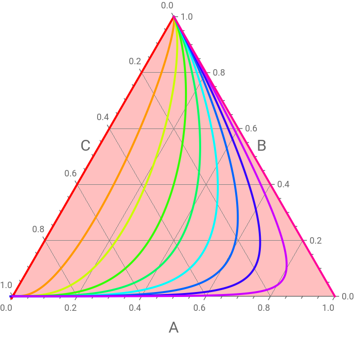
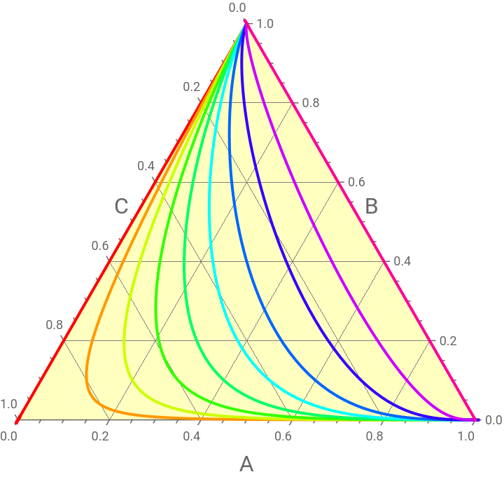
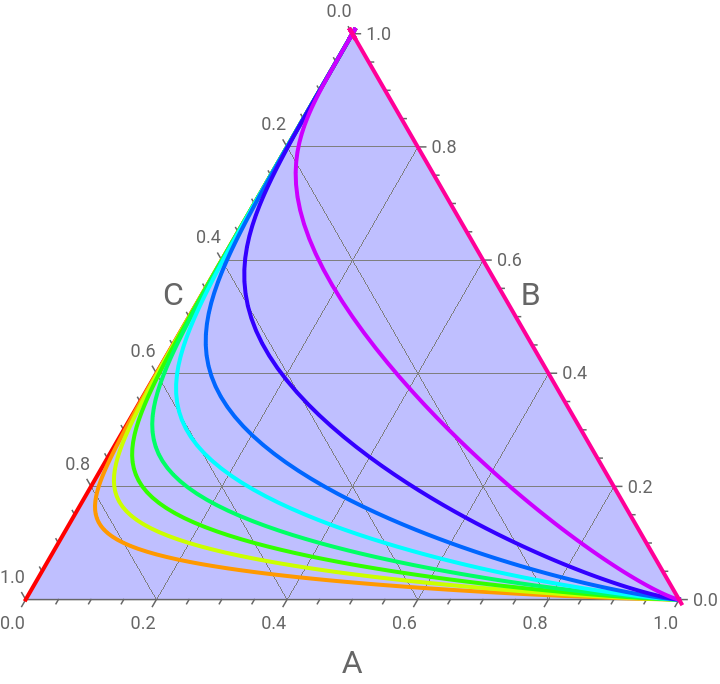
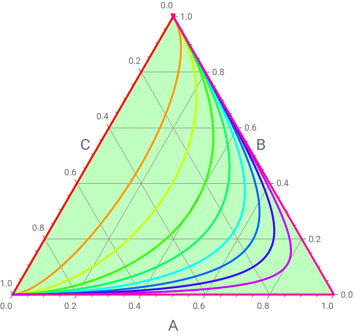
We depicts the residue curve map in an equilateral-triangular ternary diagram when the relative volatilities are :
Case 1:=1.5 and =2.5.
Case 2:=0.5 and =2.5.
Case 3:=2.5 and =0.5.
Case 4:=0.5 and =0.1.
A
B
C
A
B
C
α
13
α
23
We depicts the residue curve map in an equilateral-triangular ternary diagram when the relative volatilities are :
Case 1:
α
13
α
23
Case 2:
α
13
α
23
Case 3:
α
13
α
23
Case 4:
α
13
α
23
In[]:=
Clear[x,t,i];
In[]:=
LaunchKernels[]
Out[]=
KernelObject

In[]:=
x3[t_]:=1-x1[t]-x2[t];Sol[i_]:=NDSolve[{x1'[t]x1[t]-α13x1[t]/(α13x1[t]+α23x2[t]+x3[t]),x2'[t]x2[t]-α23x2[t]/(α13x1[t]+α23x2[t]+x3[t]),x1[0]i,x2[0]0.1},{x1,x2},{t,-40,80}];
Case 1
Case 1
α
13
α
23
In[]:=
α13=1.5;α23=2.5;
In[]:=
bl=Parallelize@Table[Table[Flatten[{x1[t]/.Sol[i],x2[t]/.Sol[i],x3[t]/.Sol[i]}]/.t->a,{a,-40,80,0.1}],{i,0,0.9,0.1}];
In[]:=
TernaryListPlot[bl,Joined->True,PlotStyle->Table[{Thick,Hue[i]},{i,0,0.9,0.1}],GridLines->Automatic,Method->{"Backdrop"->Lighter[Red,.75]},FrameLabel->{Style["A",16],Style["B",16],Style["C",16]},PlotRange->All]
Out[]=
Case 2
Case 2
α
13
α
23
In[]:=
α13=0.5;α23=2.0;
In[]:=
bl=Parallelize@Table[Table[Flatten[{x1[t]/.Sol[i],x2[t]/.Sol[i],x3[t]/.Sol[i]}]/.t->a,{a,-40,80,0.1}],{i,0,0.9,0.1}];
In[]:=
TernaryListPlot[bl,Joined->True,PlotStyle->Table[{Thick,Hue[i]},{i,0,0.9,0.1}],GridLines->Automatic,Method->{"Backdrop"->Lighter[Yellow,.75]},FrameLabel->{Style["A",16],Style["B",16],Style["C",16]},PlotRange->All]
Out[]=
Case 3
Case 3
α
13
α
23
In[]:=
α13=2.5;α23=0.5;
In[]:=
bl=Parallelize@Table[Table[Flatten[{x1[t]/.Sol[i],x2[t]/.Sol[i],x3[t]/.Sol[i]}]/.t->a,{a,-40,80,0.1}],{i,0,0.9,0.1}];
In[]:=
TernaryListPlot[bl,Joined->True,PlotStyle->Table[{Thick,Hue[i]},{i,0,0.9,0.1}],GridLines->Automatic,Method->{"Backdrop"->Lighter[Blue,.75]},FrameLabel->{Style["A",16],Style["B",16],Style["C",16]},PlotRange->All]
Out[]=
Case 4
Case 4
α
13
α
23
In[]:=
α13=0.5;α23=0.1;
In[]:=
bl=Parallelize@Table[Table[Flatten[{x1[t]/.Sol[i],x2[t]/.Sol[i],x3[t]/.Sol[i]}]/.t->a,{a,-40,80,0.1}],{i,0,0.9,0.1}];
In[]:=
TernaryListPlot[bl,Joined->True,PlotStyle->Table[{Thick,Hue[i]},{i,0,0.9,0.1}],GridLines->Automatic,Method->{"Backdrop"->Lighter[Green,.75]},FrameLabel->{Style["A",16],Style["B",16],Style["C",16]},PlotRange->All]
Out[]=
CITE THIS NOTEBOOK
CITE THIS NOTEBOOK
Residue curve maps in a triangular Ternary diagram
by Housam Binous and Ahmed Bellagi
Wolfram Community, STAFF PICKS, September 27, 2025
https://community.wolfram.com/groups/-/m/t/3551294
by Housam Binous and Ahmed Bellagi
Wolfram Community, STAFF PICKS, September 27, 2025
https://community.wolfram.com/groups/-/m/t/3551294