Import model2:
In[]:=
model2=ImportString;
Create a copy model with parameter values to allow linearization:
In[]:=
modelWithVals=SystemModel[model2,<|"ParameterValues"->{"r"->22,"l"->0.2,"c"->0.0001,"k1"->False,"k2"->True},"ModelName"->"modelWithVals"|>];
Linearize:
In[]:=
model=SystemModelLinearize[modelWithVals,Method->{"SymbolicDerivative","SymbolicParameters"->{"r","l","c","k1","k2"}}];
Select the two sets of values for the boolean parameters:
In[]:=
kVals=Thread[{QuantityVariable["k1",IndependentPhysicalQuantity[""]],QuantityVariable["k2",IndependentPhysicalQuantity[""]]}->#]&/@{{False,True},{True,False}};spacemodel={#,model/.#}&/@kVals;
Parameter values, input, initial values and stop time:
In[]:=
r=22;l=0.2;c=0.0001;vi=24;initvaluevc=0;initvalueil=0;tend=0.08;
Separate the two state space models and give them parameter values:
In[]:=
rule={QuantityVariable["r",IndependentPhysicalQuantity[""]]->r,QuantityVariable["l",IndependentPhysicalQuantity[""]]->l,QuantityVariable["c",IndependentPhysicalQuantity[""]]->c};spacemodel1=spacemodel[[1,2]]/.rule;spacemodel2=spacemodel[[2,2]]/.rule;
Two sets of state matrices a1, b1 and a2, b2
In[]:=
{a1,b1,c1,d1}=Normal[spacemodel1];{a2,b2,c2,d2}=Normal[spacemodel2];x0={{initvaluevc},{initvalueil}};
Create a function that accepts the matrices and returns responses and plots:
In[]:=
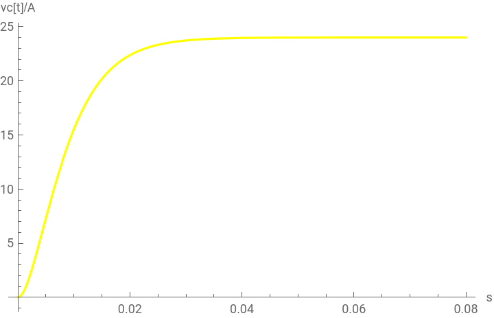
ClearAll[t,responsesAndPlots];responsesAndPlots[a_,b_]:=Module[{asi,s,τ,aA,eAt,eAtτ,x,vc,il,pvc,pil},asi=s*DiagonalMatrix[{1,1}]-a;(*MatrixA*)aA=Inverse[asi];eAt=InverseLaplaceTransform[aA,s,t];eAtτ=ReplaceAll[eAt,t->t-τ];x=eAt.x0+Integrate[eAtτ.b*vi,{τ,0,t}];(*MatrixB*)vc=x[[1,1]];il=x[[2,1]];pvc=Plot[{vc},{t,0,tend},AxesLabel{"s","vc[t]/A"},PlotLegends{"LaplaceTransform"},PlotStyle{Yellow},PlotRange->All];pil=Plot[{il},{t,0,tend},AxesLabel{"s","il[t]/A"},PlotLegends{"LaplaceTransform"},PlotStyle{Green},PlotRange->All];(*Actualfunctionoutput...herewereturnalist,butyoucanchoosewhattoreturnandinwhatformat*){vc,il,pvc,pil}]
In[]:=
responsesAndPlots[a1,b1]
Out[]=
24.+55.082-79.082,1.09091+1.02792-2.11883,
,
-267.929t
-186.617t
-267.929t
-186.617t
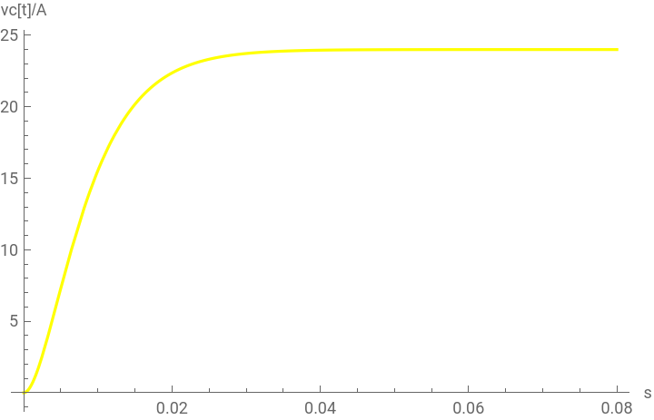

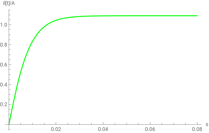

In[]:=
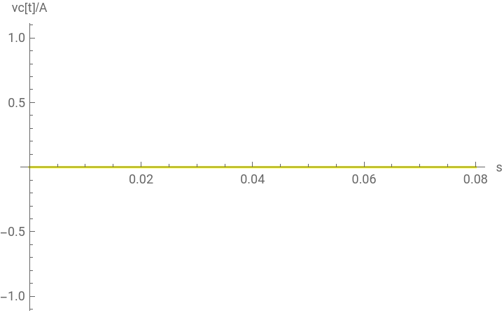
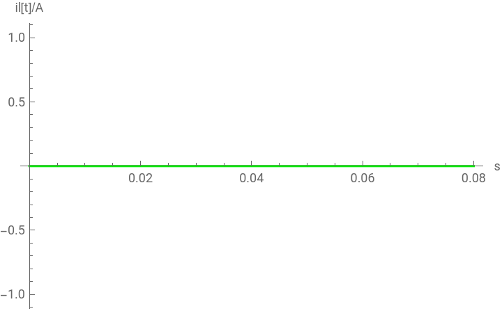
responsesAndPlots[a2,b2]
Out[]=
0.,0.,
,
But it seems that you just want to compute the state responses from the state space models and plot them. For that purpose, you can just use StateResponse which compute the responses directly from the state space models, without having to split the matrices and integrating on your own:
In[]:=
sr=StateResponse[{spacemodel1,{initvaluevc,initvalueil}},{vi},{t,0,tend}]Plot[sr[[1]],{t,0,tend},PlotRange->All,AxesLabel{"s","vc[t]/A"},PlotLegends{"LaplaceTransform"},PlotStyleYellow]Plot[sr[[2]],{t,0,tend},PlotRange->All,AxesLabel{"s","il[t]/A"},PlotLegends{"LaplaceTransform"},PlotStyleGreen]
Out[]=
InterpolatingFunction[t],InterpolatingFunction[t]


Out[]=
You can also turn this into a shorter and simpler function: