SAME MEASUREMENTS, DIFFERENT DECISION. This synthetic but scientifically representative case has 24 patients and 144 repeated measurements. Only one of the two analyses acknowledges that rows from the same patient are dependent.
The story begins at 4:45 pm. Dr Maya Nair has to brief a clinical team about a new treatment. Her file contains 144 rows, the fitted effect is 0.766, and the row-independent analysis reports p=0.0053. The decision appears easy - until she notices that the 144 rows came from only 24 people, each measured six times.
Wolfram Language has exceptionally strong tools for linear, generalized linear, nonlinear, symbolic, and probabilistic modelling. Maya's problem needs one more idea: the data remember which patient, clinic, item, animal, or instrument produced them. A native fitted-model workflow for mixed effects makes that hierarchy explicit.
This post introduces MMAMixedEffects, a native Wolfram Language paclet. Its three fitting functions follow the style of LinearModelFit and GeneralizedLinearModelFit: ordinary Wolfram expressions replace R's tilde notation, results use string properties, and fitted objects predict by function application. The current implementation covers Gaussian ML/REML models, generalized mixed models with Laplace or adaptive quadrature, nonlinear mixed models, crossed and nested factors, residual correlation, heteroscedastic variance functions, missing-row auditing, weights, offsets, Satterthwaite and Kenward-Roger inference, and a broad response-family library.
The package is tested at three levels: 275 focused Wolfram verification tests, constants-aware numerical or integral identities, and live reference fits executed with current R lme4/nlme/glmmTMB and Python statsmodels. The external languages validate the implementation; they are never called while fitting a model.
A thirty-second map
A thirty-second map
Who this is for. If you already use LinearModelFit or GeneralizedLinearModelFit and your rows come from repeated patients, schools, sites, batches, subjects, items, animals, or instruments, this post is for you. No R, Python, server, or API is required.
If you have... | Start with... |
2 minutes | patient decision + partial pooling |
5 minutes | syntax bridge + nested/crossed design |
10 minutes | GLMM, nonlinear, residual, and inference examples |
deep interest | validation and numerical architecture |
1. Setup
1. Setup
Install the attached folder as a paclet, then load its context. Readers who only want the ideas and figures can skip this section; every output is stored in the notebook.
PacletInstall[FileNameJoin[{NotebookDirectory[],"MMA MixedEffects"}]];Needs["MMAMixedEffects`"];
2. Maya's first answer - and the hidden mistake
2. Maya's first answer - and the hidden mistake
One person measured six times is not six people. Maya's treatment is assigned at patient level. Repeated rows make a naive standard error shrink as if every row were an independent randomized unit. The persistent patient-to-patient variation has not disappeared; it has simply been put into the wrong denominator.
Story provenance. Maya, her clinical team, and every patient measurement in this article are original fictional material created for this post. The data are generated by the Wolfram Language code immediately below; they are not adapted from a real patient, clinical trial, published case study, or external dataset.
patientData=Flatten[Table[With[{tr=Boole[OddQ[i]]},Table[{N[t],tr,"P"<>IntegerString[i,10,2],N[10.`+0.35`t+0.8`tr+2.2`Sin[1.33`i]+0.55`Sin[0.91`i+1.17`t]]},{t,0,5}]],{i,24}],1];
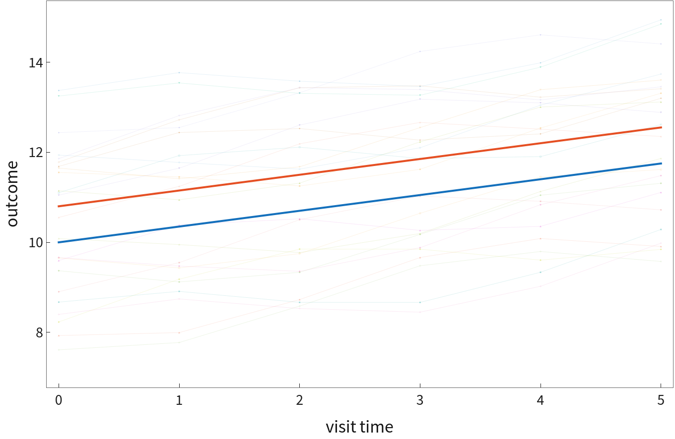
Thin lines are individual patients; thick lines are population treatment trajectories. The vertical spread is dominated by persistent patient effects, not observation noise.
Maya fits the ordinary row-level model and the patient mixed model. Both estimate the same treatment difference, 0.766. Their uncertainty is radically different. The naive calculation (equivalent to the corresponding LinearModelFit) gives SE 0.270 and p=0.0053. The patient random-intercept model gives SE 0.664 and p=0.249. Her scientific conclusion changes before a single measurement changes.
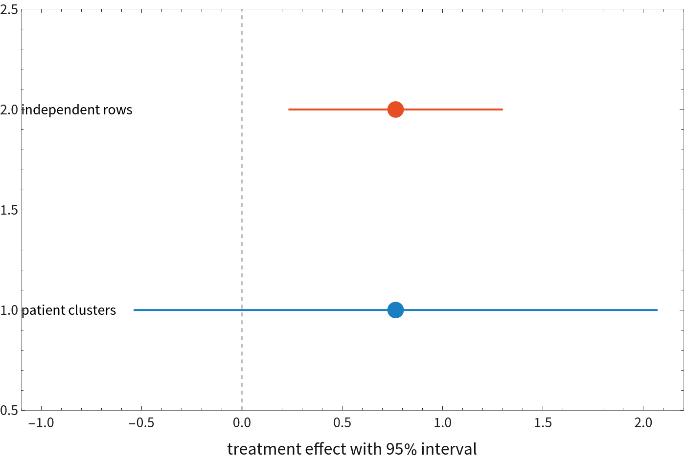
The interval from the independent-row analysis excludes zero. The interval from the hierarchical patient model crosses zero.
Decision table
Decision table
analysis | estimate | SE | p-value | decision at 5% |
LinearModelFit / independent rows | 0.7656 | 0.2701 | 0.0053 | significant |
MixedEffectsModelFit / patient clusters | 0.7656 | 0.6635 | 0.2486 | not significant |
Partial pooling
Partial pooling
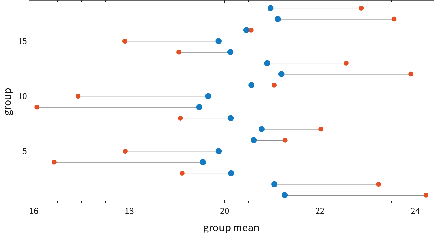
Raw patient means (orange) move toward their conditional mixed-model estimates (blue). This is shrinkage, not erasure: stable departures remain visible while noisy extremes borrow information from the population.
mu
i
w
i
mu
i
w
i
mu
The weighted compromise is the essence of partial pooling. The weight increases with within-group information and decreases when residual noise is large relative to between-group variation. Maya keeps the individuality of each patient without pretending that 24 separate small studies were performed.
The model
The model
y
ij
T
x
ij
T
z
ij
b
i
ϵ
ij
b
i
The population coefficients are shared. The vector b carries patient-, school-, site-, batch-, item-, or subject-specific departures. The residual matrix can be independent, serially correlated, spatially correlated, and heteroscedastic.
β
R
patientFit=MixedEffectsModelFit[patientData,{1,time,treatment},{{1},patient},{time,treatment,patient},Method"REML"];patientFit["ParameterTableEntries"]
3. Turning the hierarchy into a Wolfram expression
3. Turning the hierarchy into a Wolfram expression
The R expression Reaction ~ Days + (Days | Subject) is compact, but the tilde/formula language is not the normal idiom of Wolfram Language. Here the fixed and random bases are ordinary expressions:
fit=MixedEffectsModelFit[sleepData,{1,days},{{1,days},subject},{days,subject},Method"REML"];
Terms inside one random block receive a full covariance matrix. Separate blocks impose independence. A list of group specifications adds multiple factors.
fit[{"FixedEffects","RandomEffects","RandomEffectCovariances","ResidualVariance","LogLikelihood","AIC","Converged"}]
R-to-Wolfram syntax bridge
R-to-Wolfram syntax bridge
task | R formula | Wolfram Language |
fixed slope | y ~ x | {1,x} |
correlated intercept/slope | (1+x|subject) | {{1,x},subject} |
independent intercept/slope | (1|subject)+(0+x|subject) | {{{1},subject},{{x},subject}} |
crossed intercepts | (1|subject)+(1|item) | {{{1},subject},{{1},item}} |
nested intercepts | (1|site/subject) | {{{1},site},{{1},NestedGrouping[site,subject]}} |
Poisson exposure | offset(log(exposure)) | LinearOffsetFunction->Log[exposure] |
Random-structure grammar
Random-structure grammar
structure | specification | implied covariance |
correlated | {{1,x},subject} | full 2 x 2 block |
independent | {{{1},subject},{{x},subject}} | two independent blocks |
crossed | {{{1},subject},{{1},item}} | additive subject + item |
nested | {{{1},site},{{1},NestedGrouping[site,subject]}} | site + subject-within-site |
4. The study grows: clinics, patients, raters, and items
4. The study grows: clinics, patients, raters, and items
The next study is larger. Maya now has patients inside clinics and readings scored by several raters. A single patient factor no longer describes the design. Crossed effects occur when every subject may see several items and every item may be seen by several subjects. Ignoring either source of variation can make a stimulus or treatment effect look much more certain than it is.
Nested effects occur when classrooms belong to schools, samples belong to batches, or repeated plots belong to sites. The nesting is explicit rather than hidden in a formula parser:
Nested versus crossed
Nested versus crossed
A nested design is a hierarchy; a crossed design is bipartite. The list syntax mirrors that scientific distinction explicitly.
5. Time remembers: residual structure is part of the science
5. Time remembers: residual structure is part of the science
Maya has accounted for patients, but measurements taken an hour apart can still resemble each other more than measurements taken a month apart. Random effects are not a universal substitute for residual modelling. Instrument noise may increase with signal level; diets or laboratories may have different residual scales.
Residual structure in pictures
Residual structure in pictures
Left: different within-group correlation assumptions. Right: the validated BodyWeight power variance fit, where residual scale changes with time.
With MissingDataMethod->"Exclude", the fitted object retains both IncludedRowIndices and ExcludedRowIndices. Missingness is never made invisible.
The Gaussian engine supports AR(1), continuous AR(1), compound symmetry, ARMA, unstructured, exponential, Gaussian, and spherical correlations; by-level, power, exponential, constant-plus-power, and product variance functions; inverse-variance weights; offsets; and explicit missing-row exclusion.
6. The outcome changes: events, counts, and excess zeros
6. The outcome changes: events, counts, and excess zeros
At the next meeting, Maya is no longer asked how much a biomarker changed. The outcome is whether an adverse event occurred, then how many events occurred. Event probabilities, counts, positive skewed measurements, overdispersion, excess zeros, and hurdle processes require a response distribution and link. The random-effects geometry remains the same.
Three prediction targets
Three prediction targets
Population prediction sets random effects to zero; conditional prediction uses a known group's mode; marginal prediction integrates over random effects. A nonlinear link makes these curves genuinely different.
Core families are Gaussian, Binomial, Poisson, Gamma, and InverseGaussian. Advanced families include NB1/NB2/NB12, Beta, BetaBinomial, LogNormal, StudentT, and normalized zero-inflated or hurdle versions of Poisson and negative-binomial counts.
In the current constructor, the second argument of ZeroInflatedFamily or HurdleFamily is a fixed probability. It does not silently stand in for an estimated zero-part regression; validation examples say explicitly when an external zero-part MLE is supplied.
Mean-variance relationships
Mean-variance relationships
Family choice is a statement about dispersion: Poisson variance grows linearly, NB2 adds a quadratic term, and Gamma variance is proportional to the squared mean.
Laplace uses the full conditional Hessian. Adaptive Gauss-Hermite quadrature recentres and rescales nodes at the conditional mode, factors independent components, and refuses an oversized tensor grid rather than silently switching approximation. A connected crossed design can still place many latent coefficients in one component, so Laplace is usually the practical choice there.
Visible progress and less waiting
Visible progress and less waiting
Long mixed-model likelihoods should not look frozen. In a notebook, the fitting functions now show a temporary native progress panel with the current phase, marginal-objective evaluation count, best objective, active start, and elapsed time. The same calls remain silent in scripts, and no parallel kernels are launched.
Progress and benchmark
Progress and benchmark
Efficiency matters as much as feedback. The automatic generalized optimizer now begins with quasi-Newton optimization and uses deterministic Nelder-Mead only when the independent scaled-gradient audit asks for a fallback. On the live reference suite, the long binomial fits became about 20-26% faster, Poisson AGHQ about 35% faster, and Gamma about 40% faster, without changing a pass/fail result.
7. The curve bends: from recovery trajectories to Orange growth
7. The curve bends: from recovery trajectories to Orange growth
A final question is not about a straight trend at all: when does each patient approach a plateau? Growth, pharmacokinetic, decay, saturation, and learning curves differ between individuals in parameters such as asymptote, midpoint, or rate. An additive random response offset is not enough.
To keep Maya's story fictional while testing this nonlinear machinery against a transparent public benchmark, we now make one deliberate side trip to the classic Orange tree-growth data. The scientific structure is the same: repeated nonlinear trajectories, a shared population curve, and group-specific parameters. After this benchmark, the story returns to Maya's small-sample decision.
A public nonlinear benchmark: Orange growth
A public nonlinear benchmark: Orange growth
Five orange-tree trajectories and the fitted population logistic curve. Tree-specific variation acts inside the asymptote parameter.
The Wolfram expression is differentiated symbolically with D. The conditional Hessian includes the residual-times-second-derivative correction. Laplace and adaptive quadrature share the same pure likelihood path, and fixed-effect covariance comes from curvature of the marginal objective.
8. Twenty-four patients are still a small sample
8. Twenty-four patients are still a small sample
A Wald z test can be optimistic when only a handful of groups identify a fixed effect. Applicable Gaussian REML fits therefore support explicit Satterthwaite and Kenward-Roger methods:
Small-sample reference check
Small-sample reference check
The fitted entries identify the statistic type, denominator degrees of freedom, confidence level, and method. A normal approximation is never relabelled as a t test.
9. Before Maya trusts the answer: an independent model gauntlet
9. Before Maya trusts the answer: an independent model gauntlet
A reassuring plot is not evidence that an optimizer is right. A feature is not considered implemented merely because an option is accepted. It must alter the documented likelihood, expose diagnostics, pass focused mathematical tests, and agree with an independent implementation or direct integration on an appropriate model.
Five labelled release gates report their current passed/total counts. The underlying model-by-model comparisons remain visible in the tables below.
Gaussian R comparisons
Gaussian R comparisons
Independent Python comparisons
Independent Python comparisons
Generalized and residual-structure R comparisons
Generalized and residual-structure R comparisons
The matrix includes correlated and independent random slopes, crossed Penicillin, nested Pastes, Orthodont, Rail, Dyestuff, binomial cbpp with Laplace and AGHQ, Poisson exposure with AGHQ, Gamma with estimated dispersion, compound-symmetry residuals, and BodyWeight with an estimated power variance function. lme4's nAGQ>1 discrete log-likelihood convention changes additive constants, so those rows compare estimates while normalized likelihood constants are checked independently.
Twenty-three core validated configurations
Twenty-three core validated configurations
Eighteen additional documentation-derived models
Eighteen additional documentation-derived models
A second release matrix adds exactly six models for each public fitter. Gaussian examples cover Machines, Oats, Pixel, Ovary AR(1), Wafer nesting, and Dietox growth. Generalized examples cover two cbpp encodings, binary and Poisson AGHQ, and paired Salamanders Poisson/NB2 fits. Nonlinear examples cover plant physiology, pharmacokinetics, enzyme kinetics, a boundary variance, and 50 individual growth curves.
The nonlinear rows are labelled QUALIFIED_PASS because nlme's PNLS estimator and this paclet's normalized marginal Laplace objective are not identical estimators. Their release gate is based on convergence, conditional curves, residual variance, likelihood, parameters, and boundary-safe covariance differences; the label prevents estimator agreement from being advertised as parameter identity.
10. Numerical architecture: what happens underneath
10. Numerical architecture: what happens underneath
Generalized and nonlinear conditional objectives are pure; a likelihood value cannot depend on evaluation order. Quadrature uses log-sum-exp. Zero-variance boundaries are legal statistical estimates. Optimizer termination, scaled gradient quality, conditional-mode convergence, and statistical singularity are reported separately.
Automatic Gaussian and generalized fitting begins with quasi-Newton optimization and invokes deterministic Nelder-Mead refinement only when the independent gradient audit is not met. On the difficult Wafer nested-polynomial reference, this moved the fit from a false convergence failure at the same optimum to a reliable scaled gradient of 2.45*10^-6 and reduced the run from about 722 to 417 seconds.
11. Documentation that behaves like Wolfram documentation
11. Documentation that behaves like Wolfram documentation
The paclet contains six canonical DocumentationTools symbol sources and a guide. PacletDocumentationBuild transforms them into genuine in-product Documentation Center pages with anchor bars, context headers, usage signatures, Details and Options, true option tables, evaluated plots and results, Basic Examples, standard extended-example sections, cross-links, history, and search metadata.
The refreshed evaluated demonstration notebook presents more than fifteen feature examples, the twenty-three-model core zoo, and eighteen additional documentation-derived checks. PDF release artifacts are rendered to images and inspected page by page, so an empty graph or message-filled output is a release failure.
12. The decision at 5:15 pm
12. The decision at 5:15 pm
Maya returns to the clinical team with a more cautious answer: the point estimate is promising, but this experiment does not establish a treatment effect once the patient is treated as the experimental unit. She also brings something more useful than a corrected p-value: patient-specific estimates, an explicit account of residual dependence, and a model that can grow with the next study.
Mixed effects are useful whenever the data have memory of where they came from: a patient, school, site, batch, item, animal, instrument, region, or individual growth curve. Modelling that origin changes uncertainty, enables partial pooling, and can change the scientific decision.
The most important design choice is not a new syntax trick. It is making hierarchy a first-class Wolfram expression and returning a fitted object that behaves like the rest of the language.
Your first fit in five lines
Your first fit in five lines
Before interpreting a result: inspect convergence, singularity, warnings, grouping levels, residual structure, and the chosen prediction target. Then try the same workflow on one of your own clustered datasets and compare it with the row-independent analysis.
13. References
13. References
Bates, D., Maechler, M., Bolker, B. & Walker, S. (2015). Fitting Linear Mixed-Effects Models Using lme4. Journal of Statistical Software 67(1).
Pinheiro, J. & Bates, D. (2000). Mixed-Effects Models in S and S-PLUS. Springer.
Kristensen, K. et al. (2016). TMB: Automatic Differentiation and Laplace Approximation. Journal of Statistical Software 70(5).
Satterthwaite, F. E. (1946). An Approximate Distribution of Estimates of Variance Components. Biometrics Bulletin.
Kenward, M. G. & Roger, J. H. (1997). Small Sample Inference for Fixed Effects from Restricted Maximum Likelihood. Biometrics.
14. Acknowledgements
14. Acknowledgements
The implementation was independently checked against readable source and live results from lme4, nlme, glmmTMB, lmerTest, pbkrtest, and statsmodels. The cover animation and all figures were generated in Wolfram Language from the evaluated examples; no external image generator was used.
15. Reproducibility
15. Reproducibility
The attached paclet contains kernel source, focused verification tests, data files, R and Python reference runners, Wolfram live runners, exact comparison tolerances, evaluated documentation, this Community notebook, and the PDF/visual verification workflow. R and Python are optional validation dependencies only.
CITE THIS NOTEBOOK
CITE THIS NOTEBOOK
Mixed effects models: when 144 measurements are only 24 patients
by Marco Thiel
Wolfram Community, STAFF PICKS, August 5, 2026
https://community.wolfram.com/groups/-/m/t/3774128
by Marco Thiel
Wolfram Community, STAFF PICKS, August 5, 2026
https://community.wolfram.com/groups/-/m/t/3774128