ABSTRACT (original article): We study implications of Leibnizian ideas such as the identity of indiscernibles, and variety (due to Barbour and Smolin) in the context of Wolfram Model, which has been put forward in 2020. We have provided (at the moment) speculative interpretations for Leibnizian and non-Leibnizian hypergraphs. We introduced an action based on variety, to select paths where it is maximized. The specific universe which is of concern here is the one with name ‘wm1268’ from the Registry of Notable Universe Models, which is used as a test case in the present study. CITATION (original article): Dündar, F.S. A Case Study for Leibnizian Ideas in Wolfram Model. Found Phys 54, 43 (2024). https://doi.org/10.1007/s10701-024-00777-3
Required Software
Required Software
First we need to install the SetReplace packet from https://github.com/maxitg/SetReplace In order to install this package, please refer to its website.
Second we need to install the Variety packet from https://github.com/fsdundar/wolfram-model-variety/ In order to use this package, it would be enough to place the Variety.wl file in the same directory of this Mathematica Notebook.
Now we import these packages.
In[]:=
SetDirectory[NotebookDirectory[]];
In[]:=
<<SetReplace`
In[]:=
<<Variety`
Now we are ready to move forward.
Introduction
Introduction
In this notebook we consider the wm2117 model universe from the Registry of Notable Universes. (In the published article the universe model is wm1268). By modifying the following variable, you can study other universe models easily.
In[]:=
uniNumber=2117;
The initial state and re-write rule of wm2117 are given as:
In[]:=
init=ResourceFunction["WolframModelData"][uniNumber,"InitialCondition"]
Out[]=
{{1,1,1},{1,1,1}}
In[]:=
rwRule=ResourceFunction["WolframModelData"][uniNumber,"Rule"]
Out[]=
{{{1,2,2},{3,1,4}}{{4,1,1},{5,3,4},{5,2,3}}}
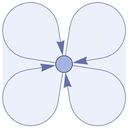
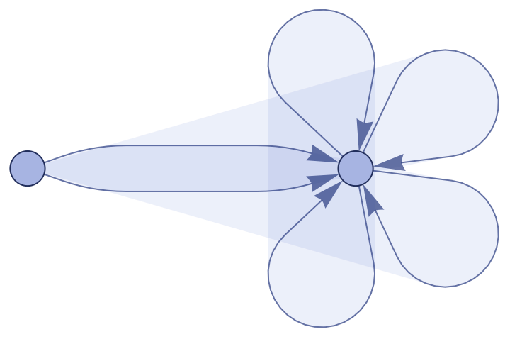
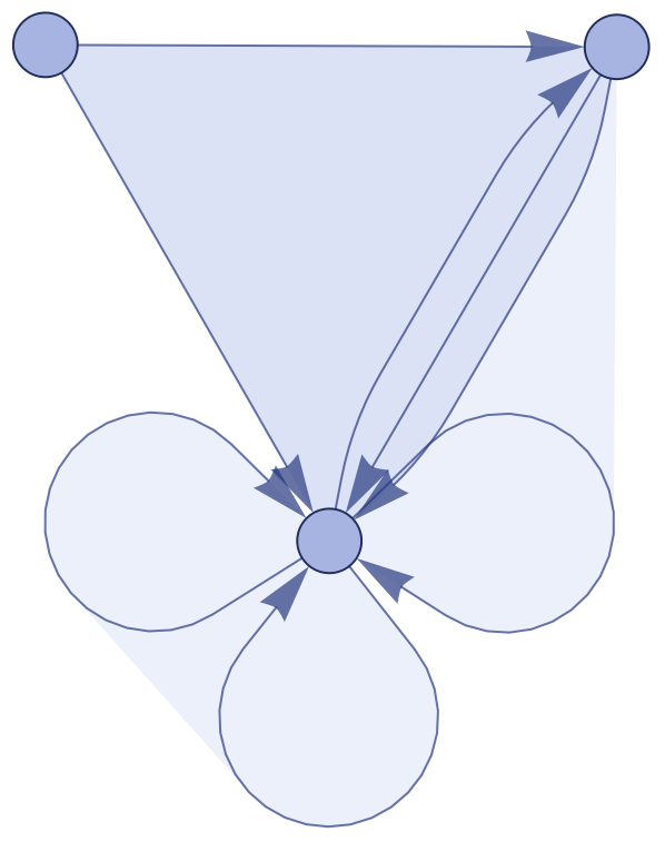
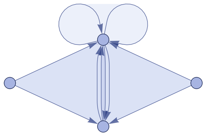
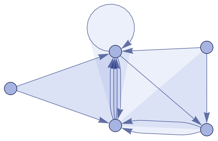
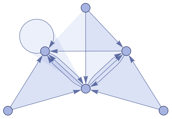
Let us plot its initial Wolfram Model evolution:
In[]:=
WolframModel[rwRule,init,7,"StatesPlotsList"]
Out[]=
,
,
,
,
,
,
,
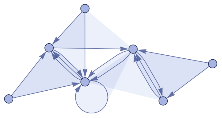
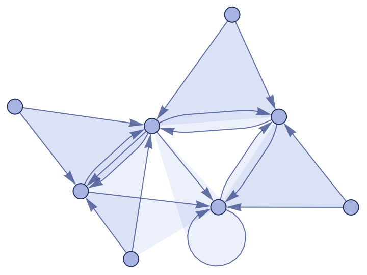
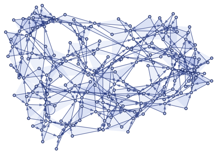
Here we plot the configuration of this universe model after 200 time steps.
In[]:=
WolframModel[rwRule,init,200,"FinalStatePlot"]
Out[]=
Let us calculate the BSD variety of these hypergraphs:
In[]:=
global7=WolframModel[rwRule,init,7,"StatesList"];
In[]:=
global7vars=Variety/@global7
Out[]=
0,2,3,0,5,,6,
14
3
13
2
Then we plot the variety values:
In[]:=
ListLinePlot[global7vars,Mesh->Full,AxesLabel->{"Depth","Variety"}]
Out[]=
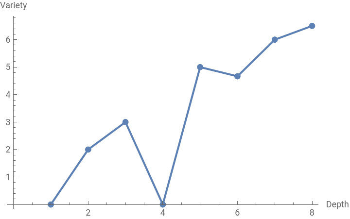
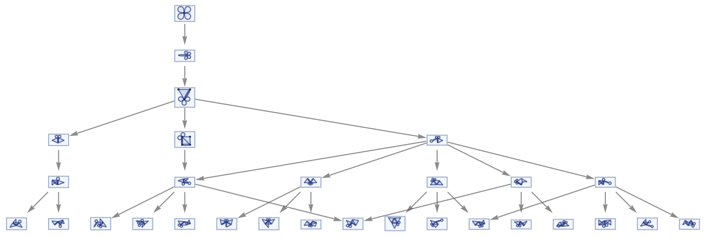
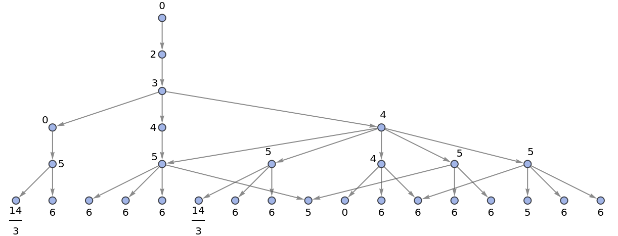
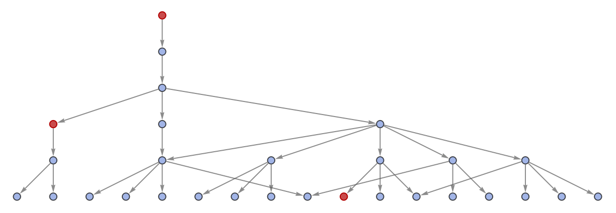
The configurations with zero variety are non-Leibnizian. Later we will see that there is a way to move around these configurations in the multiway system of Wolfram Model, similar to the idea of analytical continuation. (For an illustration of this idea, please refer to Figure 7 in the paper). Let us now move on to the multiway system for this universe. The following graph is the beginning of the multiway system associated with this universe.
In[]:=
ResourceFunction["MultiwaySystem"]["WolframModel"->rwRule,{init},5,"StatesGraph",Sequence[VertexSize->1,GraphLayout->"LayeredDigraphEmbedding"],ImageSize->Large]
Out[]=
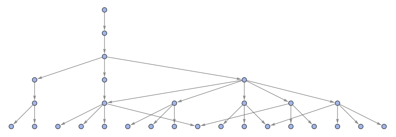
Because we will not be interested in actual configurations but their BSD variety values, we define the following multiway system.
In[]:=
mw5=ResourceFunction["MultiwaySystem"]["WolframModel"->rwRule,{init},5,"StatesGraphStructure",Sequence[VertexSize->0.2,GraphLayout->"LayeredDigraphEmbedding"],ImageSize->Large]
Out[]=
BSD Variety of Hypergraphs
BSD Variety of Hypergraphs
We now calculate the BSD variety of each configuration and put them near each vertex on the multiway system.
In[]:=
hgs5=VertexList[mw5];
In[]:=
vars5rule=#->Variety[#]&/@hgs5;
In[]:=
Graph[mw5,VertexLabels->vars5rule]
Out[]=
In[]:=
nonLeibnizianQ[hg_]:=(hg/.vars5rule)==0
In[]:=
hgs5nonLeibnizian=Select[hgs5,nonLeibnizianQ];
Red vertices in the following graph are non-Leibnizian.
In[]:=
HighlightGraph[mw5,hgs5nonLeibnizian,ImageSize->Large]
Out[]=
Paths in the Multiway System
Paths in the Multiway System
In this section, we will calculate various paths in the multiway system. We begin by calculating the vertices in the multiway system.
Because the first node is non-Leibnizian, we will calculate paths emanating from the second vertex.
We now calculate all the paths in the multiway system.
The action of a path, is the sum of all BSD variety values. If there is a non-Leibnizian hypergraph along the path, we set its action to zero.
We now find the maximum action.
Let us now define a few functions that will be useful.
Physical paths are defined on the multiway system such that all the vertices it passes on are Leibnizian (positive BSD variety).
Maximum action paths are physical paths such that the sum of BSD variety is maximized.
Paths Highlighted in the Multiway System
Paths Highlighted in the Multiway System
We now combine the various paths found in the last section into a graph structure.
Here we highlight these (sub)graphs in the multiway system. This is the graph of physical paths:
This is the graph of maximum action paths:
Conclusion
Conclusion
In this Mathematica Notebook, we illustrated the main algorithms and ideas in our paper published in the journal of Foundations of Physics. For a more comprehensive understanding of the calculations presented here and their interpretations please refer to the paper mentioned.
CITE THIS NOTEBOOK
CITE THIS NOTEBOOK
A case study for Leibnizian ideas in Wolfram Model
by Furkan Semih Dündar
Wolfram Community, STAFF PICKS, July 5, 2024
https://community.wolfram.com/groups/-/m/t/3205962
by Furkan Semih Dündar
Wolfram Community, STAFF PICKS, July 5, 2024
https://community.wolfram.com/groups/-/m/t/3205962