S23Parameter solution for mean
S23Parameter solution for mean
It turns out that the mu parameter for the S23OrderDistribution carries the information about the distribution expectation, but to extract it requires the other three parameters, {alpha, beta, sigma}. There does not appear to be a simple closed formula, and it also appears that when doing the calculations, the zero parameterization for the distribution has a simpler curve.
In[]:=
Needs["S23OrderDistribution`"]
mu is the mean of the distribution when beta = 0, and the distribution is symmetric. This is true in both the 0 and 1 parameterizations, which are the same when beta is zero.. In the graph below mu is 5, alpha is 2.8. For any given alpha the relation ship is linear but the slope is different.
In[]:=
bmn=Quiet@Table[{b,NIntegrate[xPDF[S23OrderDistribution[2.8,b,5,1,0],x],{x,-∞,∞}]},{b,-1,1,0.2}];ListPlot[%]
Out[]=
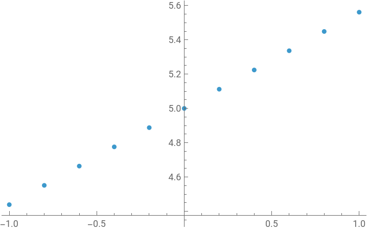
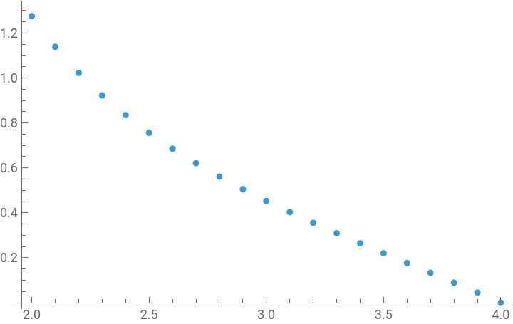
These slopes can be determined numerically by fitting the points above to a line, and then calculated for a large set of alpha to get an interpolation function. Below are the results for alpha [2,4] where most stock market return distributions lie. It was computed using the above integral for the range of alpha, and takes quite a while. The Z in the names is to remind me that it is the zero parameterization.
In[]:=
alphaDataZ={{2.`,1.2751430177330012`},{2.1`,1.1384745147939086`},{2.2`,1.02229132823788`},{2.3`,0.9220919997537144`},{2.4`,0.834180048769181`},{2.5`,0.7558770911787418`},{2.6`,0.685191638051022`},{2.7`,0.6206079980377776`},{2.8`,0.5609476514556675`},{2.9`,0.5052742304830133`},{3.`,0.4523763243561142`},{3.1`,0.4029881755080235`},{3.2`,0.355218446079988`},{3.3`,0.3090626340227001`},{3.4000000000000004`,0.26411384724977044`},{3.5`,0.22000313645061143`},{3.6`,0.1763826692903297`},{3.7`,0.13291520224935385`},{3.8`,0.08926540671038571`},{3.9000000000000004`,0.04508424665619868`},{4.`,0.}};
In[]:=
ListPlot[alphaDataZ]
Out[]=
In[]:=
alphaFnZ=Interpolation[alphaDataZ]
Out[]=
InterpolatingFunction


Formula for the mean.
Formula for the mean.
In[]:=
s23meanZ[alpha_,beta_,mu_,sigma_]:=mu+betasigmaalphaFnZ[alpha];
In[]:=
{alpha,beta,mu,sigma}={2.9,0.5,3,1}
Out[]=
{2.9,0.5,3,1}
In[]:=
NIntegrate[xPDF[S23OrderDistribution[alpha,beta,mu,sigma,0],x],{x,-∞,∞}]s23meanZ[alpha,beta,mu,sigma]
Out[]=
3.25246
Out[]=
3.25264
Market simulation
Market simulation
Here are stock market parameters for KLAC for the past two years in the zero parameterization.
In[]:=
{"KLAC",{2.275947950575399`,-0.07798724676835758`,0.004180537368125536`,0.0245680092683324`,0}};klac=Most[%[[2]]]
Out[]=
{2.27595,-0.0779872,0.00418054,0.024568}
In[]:=
kmn=s23meanZ[Sequence@@klac]
Out[]=
0.00237006
That gives the average trading day return. There about 250 trading days per year so that would be an annual decimal return over the past two years of:
In[]:=
Exp[250kmn]-1
Out[]=
0.808531
In[]:=
S23OrderDistribution[Sequence@@klac,0]
Out[]=
S23OrderDistribution[2.27595,-0.0779872,0.00418054,0.024568,0]
In[]:=
klacrv=RandomVariate[S23OrderDistribution[Sequence@@klac,0],500];ListPlot[80Exp[FoldList[Plus,0,klacrv]],PlotRange->All,PlotLabel->"KLAC Price Simulation"]
Out[]=
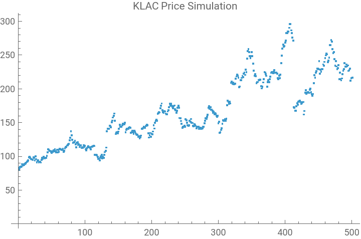
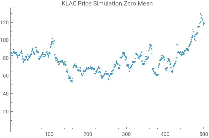
The simulation obviously is carrying the mean of the distribution. Here is a zero mean simulation.
In[]:=
Clear[mu]parm=ReplacePart[klac,3->mu]
Out[]=
{2.27595,-0.0779872,mu,0.024568}
In[]:=
mu0=mu/.FindRoot[s23meanZ[Sequence@@parm]==0,{mu,0.002}]
Out[]=
0.00181048
In[]:=
parm1=parm/.mu->mu0
Out[]=
{2.27595,-0.0779872,0.00181048,0.024568}
In[]:=
klacrv=RandomVariate[S23OrderDistribution[Sequence@@parm1,0],500];ListPlot[80Exp[FoldList[Plus,0,klacrv]],PlotRange->All,PlotLabel->"KLAC Price Simulation Zero Mean"]
Out[]=
Calculating the mean by numerical integration can be time consuming. The first point for the interpolation function took 20 minutes on an older desk top. More points could be added to the grid for better accuracy, but for most purposes with financial returns the current version should be good enough.