This is one of the interesting problems proposed by Stanley Rabinowitz. It was published on Fibonacci Quarterly (Aug. 1988 H283). Regardless of the simple statement, using modern technology, the visualization of the root location is very beautiful and pleasing.
Out[]=

Let’s formulate the LHS of the equation with the following code. Note that the coefficient parts are just vanilla Fibonacci function from n to 2n, yet the degree of each x term is descending from n to 0 correspondingly. To have both Fibonacci terms and x terms share the same index k for summation, it is wise to use so that the descending degrees match the ascending indices in Fibonacci coefficients.
(2n-k)
x
In[]:=
fibPoly[n_Integer]:=Sum[Fibonacci[k]*x^(2n-k),{k,n,2*n}]
Though I call it fibPoly, it has nothing to do with actual Fibonacci Polynomial Fibonacci[n,x], a function defined in WL.
For example, when , we have a tenth degree polynomial whose coefficients are from 10th term to 20th term in the Fibonacci sequence
n10
In[]:=
poly=fibPoly[10]
Out[]=
6765+4181x+2584+1597+987+610+377+233+144+89+55
2
x
3
x
4
x
5
x
6
x
7
x
8
x
9
x
10
x
Solve/NSolve is able to locate all roots for polynomial. Solve returns symbolic results in the form of root object
In[]:=
RandomSample[x/.Solve[poly==0,x],1][[1]]
Out[]=

In[]:=
{Accuracy[#],Precision[#]}&@%
Out[]=
{∞,∞}
NSolve returns numeric values in machine precision by default, which is enough for my application here.
In[]:=
roots=x/.NSolve[poly==0,x];
ComplexListPlot shows a simple scattered diagram of the location of the roots on a complex plane.
In[]:=
ComplexListPlot[roots]
Out[]=
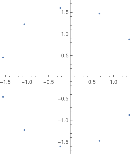
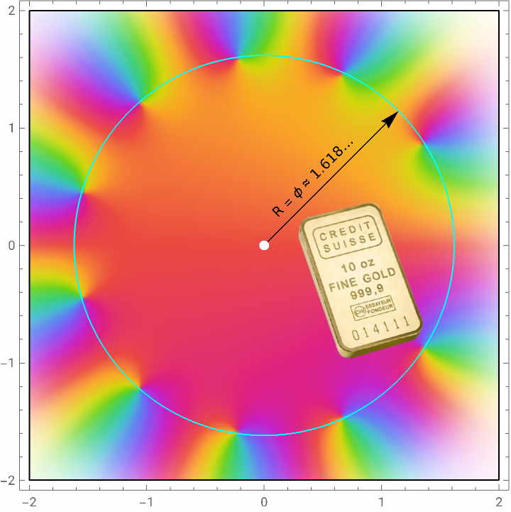
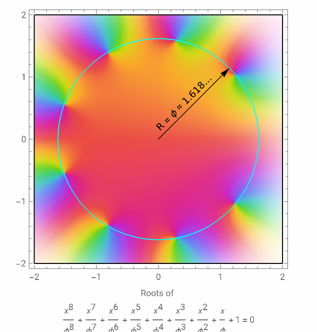
If you need more intriguing visualization about the function behavior around roots in terms of magnitudes and argument, you can use ComplexPlot. The brighter, the larger the magnitude of the function. The rainbow color indicated the principle argument of the function. If I overlay a circle centered at the origin and with radius equal to the golden ratio, the roots indeed look like sitting on the circle.
In[]:=
ManipulateComplexPlotfibPoly[n],{x,2},Epilog,{n,1,15,1},SaveDefinitionsTrue
Out[]=

Sketch of the Proof
Sketch of the Proof
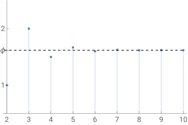
The rigorous proof is found in the “Advanced Problems and Solutions” in Fibonacci Quarterly Aug 1990 Vol. 28. I can quickly summarize what is happening in the manual. The basic idea is that the ratio of the consecutive terms in Fibonacci sequence approaches the golden ratio fairly quickly. This can be checked both visually and symbolically in WL.
In[]:=
DiscretePlot,{n,2,10},
Fibonacci[n]
Fibonacci[n-1]
Out[]=
In[]:=
Limit,n->Infinity
Fibonacci[n]
Fibonacci[n-1]
Out[]=
1
2
5
)Also we know that and so on for any in integer. Thus we know the above limit for Fibonacci with terms apart must be . Thus if we divide on the both sides of +++...x+0 , for large , we have something very close to a geometric progression in terms of
f(n)
f(n-2)
f(n)
f(n-1)
f(n-1)
f(n-2)
n-k
k
k
ϕ
F
2n
F
n
n
x
F
n+1
n-1
x
F
n+2
n-2
x
F
2n-1
F
2n
n
(x/ϕ)
In[]:=
goldenPoly[n_]:=
2n
∑
k=n
2n-k
x
GoldenRatio
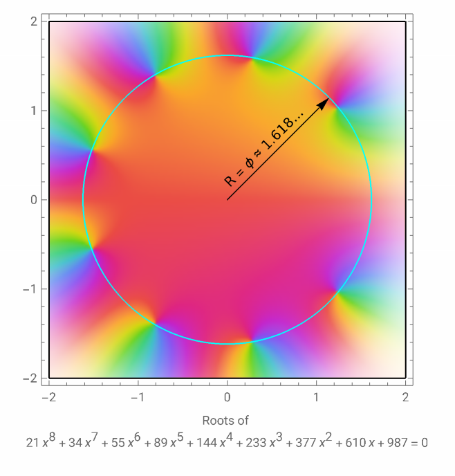
To prove the original statement, we come up a stronger version, roughly speaking: the location of roots of my goldenPoly[n] is the limit of those of my fibPoly[n]. Visually, it means the left plot and right plot are almost the same.
In[]:=
padding={{30,30},{65,10}};GridComplexPlotfibPoly[8],{x,2},,ComplexPlotgoldenPoly[8],{x,2},
Out[]=
The idea, illustrated below, is that moves the pole continuously between the poles of and that of .
(1-t)goldenPoly[n]+tfibPoly[n]
g
f
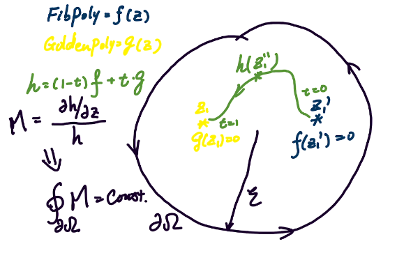
Define M function is to check the Cauchy contour integral to count the number of poles in the closed region
In[]:=
m[n_,t_]:=
D[(1-t)goldenPoly[n]+t*fibPoly[n],x]
(1-t)goldenPoly[n]+t*fibPoly[n]
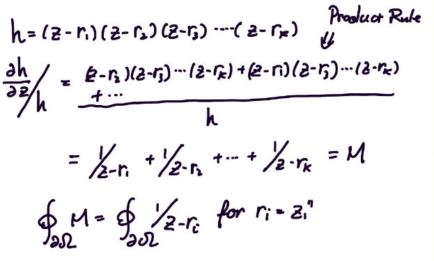
Note that is also a polynomial, so we can use the fundamental theorem of algebra and product rule of differentiation to find the contour integral of M
h
Take a look at the vicinity of the root for both goldenPoly and fibPoly.
Move t from 0 to 1 we see M function is invariant when integrated along a small circle including the chosen root.
Summary
Summary
◼
ComplexPlot gives detailed behaviour for complicated functions
◼
Limit and Fibonacci function works well together to verify the adjacent term ratio limit
◼
DiscretePlot works well with visual check of convergence
◼
The documented variable replace trick is useful for NIntegrate on complex domain
◼
Manipulate is really handy to create the animation at the beginning
◼
Understanding Cauchy integral and uniform continuity is required for the formal proof. Otherwise, intuition matches the expected result.