This notebook shows the numerical inversion of Laplace transforms using Herbert E. Salzer's method [1] and uses functions by Jan Mangaldan (https://tpfto.wordpress.com/2012/05/04/quick-and-dirty-inversion/).Herbert E. Salzer’s method allows the determination of for a given as follows:, where are the roots of (-n,n;_;z), =({1-n,n-1};{};) are the Christoffel numbers, and (a;b;z) are the generalized hypergeometric functions.Case 1:The test function is , where . The exact inverse Laplace transform is given by , where is the Bessel function of the first kind of order zero. The error (i.e. the difference between the exact inverse and the numerical inverse) is also given. The numerical method fails at large and can only serve as a quick-and-dirty technique for the inversion of Laplace transforms.Case 2:The test function is , where . The exact inverse Laplace transform is given by . Again, the method fails at large t.Case 3:The test function is , where . The exact inverse Laplace transform is given by . Again, the method fails at large t.[1] H. E. Salzer, “Orthogonal Polynomials Arising in the Numerical Evaluation of Inverse Laplace Transforms,” Mathematics of Computation, 9(52), 1955 pp. 164–177. doi: 10.1090/S0025-5718-1955-0078498-1.
f(t)
F(s)=ℒ(f(t))(s)
f(t)=F(p)dp=Ft
1
2πj
c+j∞
∫
c-j∞
pt
e
n
∑
i=1
1
t
(n)
A
i
1
p
i
z=
p
i
2
F
0
(n)
A
i
n+1
(-1)
p
i
n
2
2n-1
2
F
0
p
i
p
F
q
F(s)=ℒ(f(t))=+
1
2
a
2
s
a=1
f(t)=(at)
J
0
J
0
t
F(s)=ℒ(f(t))=
1
2
s
2
(1+as)
a=1
f(t)=t-2a+(1+2a)
-t/a
F(s)=ℒ(f(t))=+
s
2
s
2
a
a=4
f(t)=cos(at)
Case 1
Case 1
In[]:=
a=1;
In[]:=
SalzerRuleData[n_Integer,prec_:MachinePrecision]:=Block[{x},Transpose[Map[{#,(-1)^(n+1)#((2n-1)/HypergeometricPFQ[{1-n,n-1},{},#])^2/n}&,x/.NSolve[HypergeometricPFQ[{-n,n},{},x],x,prec]]]];NInverseLaplaceTransform[f_,s_,t_,opts:OptionsPattern[]]:=Module[{xa,wt},{xa,wt}=SalzerRuleData[10,MachinePrecision];Chop[(wt.Function[s,f][1/xa/t])/t]];
In[]:=
f[t_]=NInverseLaplaceTransform[1/Sqrt[a^2+s^2],s,t,WorkingPrecision25]//Chop;g[t_]:=InverseLaplaceTransform[1/Sqrt[a^2+s^2],s,t];
In[]:=
Plot[{f[t]//Chop,g[t]},{t,0,20},FrameTrue,GridLinesAutomatic,AspectRatio1,PlotStyle{{Red,Thick},{Blue,Dashed,Thick}},ImageSize350{1,1}]
Out[]=
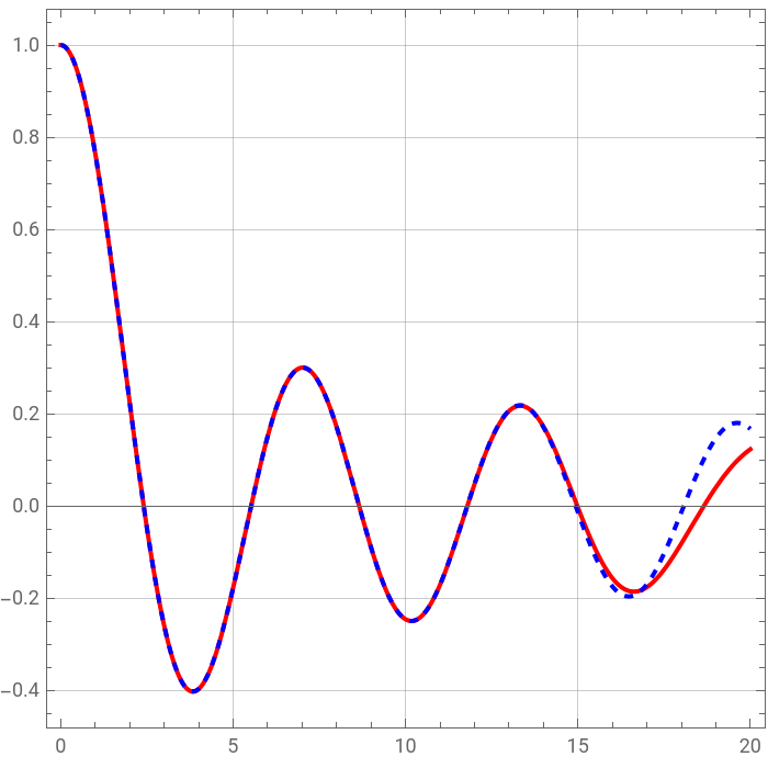
In[]:=
Plot[f[t]-g[t]//Chop,{t,0,20},FrameTrue,PlotRangeAll,AspectRatio1,PlotStyle{Magenta,Thick},GridLinesAutomatic,ImageSize350{1,1}]
Out[]=
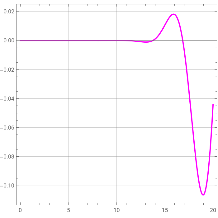
In[]:=
a=4.9;
In[]:=
f[t_]=NInverseLaplaceTransform[1/Sqrt[a^2+s^2],s,t,WorkingPrecision25]//Chop;g[t_]:=InverseLaplaceTransform[1/Sqrt[a^2+s^2],s,t];
In[]:=
Plot[{f[t]//Chop,g[t]},{t,0,10},FrameTrue,GridLinesAutomatic,AspectRatio1,PlotStyle{{Red,Thick},{Blue,Dashed,Thick}},ImageSize350{1,1}]
Out[]=
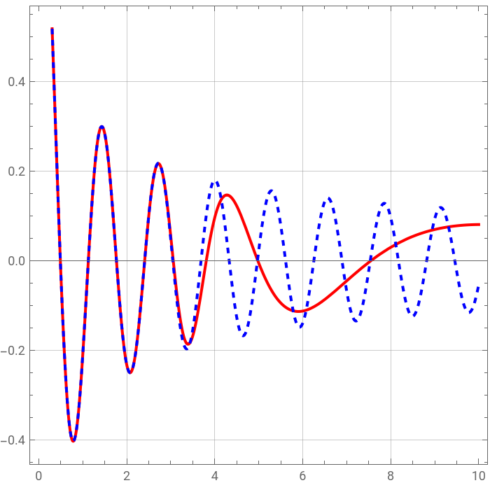
Case 2
Case 2
In[]:=
f[t_]=NInverseLaplaceTransform[1/s^2/(as+1)^2,s,t,WorkingPrecision25]//Chop;g[t_]:=InverseLaplaceTransform[1/s^2/(as+1)^2,s,t];
In[]:=
Plot[{f[t]//Chop,g[t]},{t,0,7},FrameTrue,GridLinesAutomatic,AspectRatio1,PlotStyle{{Red,Thick},{Blue,Dashed,Thick}},ImageSize350{1,1}]
Out[]=
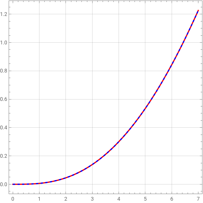
Case 3
Case 3