Abstract: In this project, the concept of Newton Polytopes is studied in the light of Tropical Geometry using the MinPlus algebra. The Newton Polytopes are visualized using Plot3D, and tropical curves can be visualized using ContourPlot. A two dimensional method of creating the tropical curves has been studied before whereas 3D method is easier to code and visualize. In this notebook, first we convert an algebraic polynomial into a tropical polynomial using MinPlus algebra, then we will extract the 3D coordinates to draw the Newton Polytope. This is an introductory level project in Tropical Geometry that can be further extended to other related fields like Physics and Economics.
Tropical Geometry
Tropical Geometry
Tropical Geometry is a relatively new field which deals with combinatorics and algebraic geometry. It involves a degeneration of algebraic varieties into tropical varieties, which is called tropicalization[1]. Tropical Geometry has been a successful tool for studying enumerative problems.
A Newton Polytope is an integral polytope associated with a multivariate polynomial. The Newton Polytope can be used to study the polynomial's behavior when certain variables are considered negligible relative to the others. We have studied the three-dimensional Extended Newton Polytopes associated with tropical polynomials using the MinPlus tropical algebra defined over the tropical Semiring. In this project, we have implemented a process that takes a tropical polynomial as an input and returns the associated Newton polytope.
A Newton Polytope is an integral polytope associated with a multivariate polynomial. The Newton Polytope can be used to study the polynomial's behavior when certain variables are considered negligible relative to the others. We have studied the three-dimensional Extended Newton Polytopes associated with tropical polynomials using the MinPlus tropical algebra defined over the tropical Semiring. In this project, we have implemented a process that takes a tropical polynomial as an input and returns the associated Newton polytope.
Tropical Semiring
Tropical Semiring
The tropical semiring is defined as ℛ = ( ⋃ {∞}, ⊕, ⊗),where ⊕ is the usual minimum, and ⊗ is the usual addition. The operations are associative, distributive and commutative. Here, 0 is the multiplicative identity and ∞ is the additive identity. There is only one ring axiom that does not work: there is no tropical subtraction. These operations are written as MinPlus algebra and in the following example, we will take a polynomial and apply some MinPlus algebra on it.
For example:
In[]:=
p=8x+2y+5(*amultivariatepolynomial*)
Out[]=
5+8x+2y
In[]:=
MinPlus[poly_]:=ReplaceAll[poly,(*ThisfunctiontakesapolynomialasanargumentandappliestheMinPlusalgebraonit*){PlusMin,TimesPlus,PowerTimes}];
In[]:=
MinPlus[p](*appliedMinPlusalgebraonapolynomialp*)
Out[]=
Min[5,8+x,2+y]
We can visualize a two-dimensional tropical curve in a ContourPlot of the tropicalized polynomial. Here we have used the same polynomial p as above.
In[]:=
ContourPlot[MinPlus[p],{x,-5,2},{y,-2,5},ExclusionsStyleBlack]
Out[]=
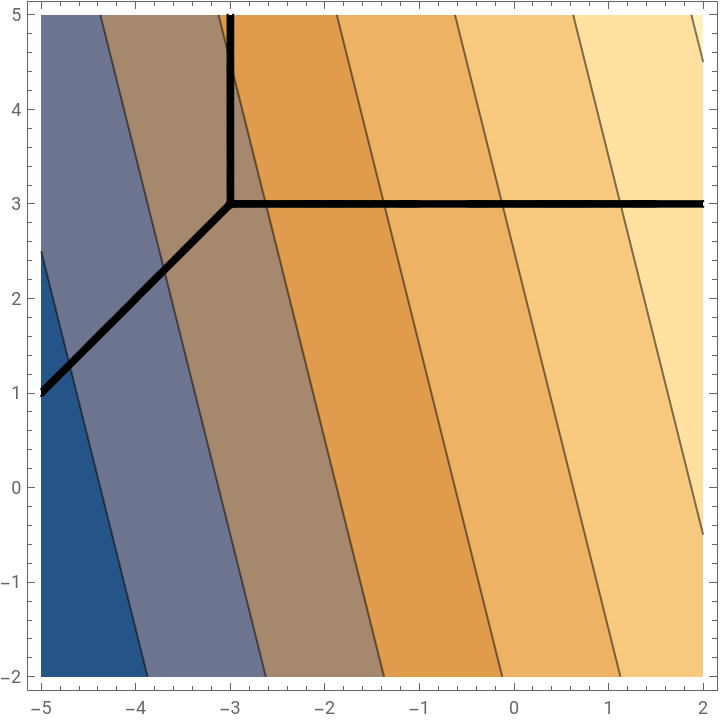
The polynomial above is now expressed using MinPlus algebra.
Q. Why are we not using one-variable polynomials?
A. An algebraic polynomial in one variable corresponds to a 2D graph and a tropical polynomial in one variable corresponds to a piecewise linear function. As I have mentioned above, we are investigating Newton Polytopes, which require hypersurfaces as an input (multivariable function). Therefore, we will be using a multivariable rather than one-variable function.
Q. Is the definition correct?
A. Yes. The above function simply takes a polynomial, applies MinPlus algebra and gives a polynomial in algebraic geometry. However, for tropical geometry, the form of tropical polynomial is a little bit different in terms of the coefficients. I will explain what a tropical polynomial is in the next section.
Q. Why are we not using one-variable polynomials?
A. An algebraic polynomial in one variable corresponds to a 2D graph and a tropical polynomial in one variable corresponds to a piecewise linear function. As I have mentioned above, we are investigating Newton Polytopes, which require hypersurfaces as an input (multivariable function). Therefore, we will be using a multivariable rather than one-variable function.
Q. Is the definition correct?
A. Yes. The above function simply takes a polynomial, applies MinPlus algebra and gives a polynomial in algebraic geometry. However, for tropical geometry, the form of tropical polynomial is a little bit different in terms of the coefficients. I will explain what a tropical polynomial is in the next section.
Tropical Polynomial
Tropical Polynomial
Finding the coordinates of a Tropical Polynomial utilises the same definition of MinPlus algebra except that the coefficient of every term is taken from p-adic valuation. For n ∈ N, the highest power of a prime p that divides n is called the p-adic valuation of the n. For simplicity, we are taking 2-adic valuation[2].
Let's take the polynomial p,
In[]:=
p
Out[]=
5+8x+2y
8 can be rewritten as 2×2×2 the highest power of a prime 2 that divides 8 is 3 and 3 is called the 2-adic valuation of 8.
2 can be rewritten as 2×1 and the highest power of a prime 2 that divided 2 is 1 and 1 is called the 2-adic valuation of 2.
5 can be rewritten as 5×1 and the highest power of prime 2 that divides 2 is 0 and 0 is called the 2-adic valuation of 5.
The coefficients after applying the 2-adic valuation are {3, 1, 0}.
The function below computes the 2-adic valuations of the coefficients:
2 can be rewritten as 2×1 and the highest power of a prime 2 that divided 2 is 1 and 1 is called the 2-adic valuation of 2.
5 can be rewritten as 5×1 and the highest power of prime 2 that divides 2 is 0 and 0 is called the 2-adic valuation of 5.
The coefficients after applying the 2-adic valuation are {3, 1, 0}.
The function below computes the 2-adic valuations of the coefficients:
In[]:=
valuation=IntegerExponent[#,2]&/@Last/@CoefficientRules[p,{x,y}](*thisfunctionbringsthevaluationofeverycoefficient*)
Out[]=
{3,1,0}
With the 2-adic valuation, we can write a function that converts a traditional polynomial into a tropical polynomial.
tropoly[poly_,variables_]:=Min@@(Flatten/@Transpose[{First/@CoefficientRules[poly,variables],IntegerExponent[#,2]&/@Last/@CoefficientRules[poly,variables]}].Append[variables,1])
In[]:=
tropoly[p,{x,y}]
Out[]=
Min[0,3+x,1+y]
The function tropoly applies the definition of tropicalization or tropicalizing the polynomial. If you compare the expressions we have from using MinPlus algebra and tropical polynomial, you can clearly spot the difference of the coefficients 3 instead of 8, 1 instead of 2 and 0 instead of 5. These are valuations we have calculated using the 2-adic valuation.
Newton Polytope
Newton Polytope
The Newton polytopes are drawn on three-dimensional polytope vertices.
1. Get exponent vectors
2. Get coefficients from valuation
3. Form 3D coordinates
The first two coordinates (x,y) are the exponent vectors while the z component is the coefficient extracted from 2-adic valuation. The exponent vectors of polynomial p are:
1. Get exponent vectors
2. Get coefficients from valuation
3. Form 3D coordinates
The first two coordinates (x,y) are the exponent vectors while the z component is the coefficient extracted from 2-adic valuation. The exponent vectors of polynomial p are:
1. Exponent Vectors
1. Exponent Vectors
In a two variable function f(x,y), every expression has both variables. The list of maximum powers of every variable in each expression is called the exponent vector. Lets take the polynomial p from the previous section:
In[]:=
p//TraditionalForm
Out[]//TraditionalForm=
8x+2y+5
Find its exponent vectors:
In[]:=
expvec=First/@CoefficientRules[p,{x,y}]
Out[]=
{{1,0},{0,1},{0,0}}
Now we have a list of the exponent vectors of each term in the polynomial with respect to both variables (x, y). The term 8 x has the variable x with power 1 and y with power 0, hence the first element in the list is {1 ,0}. Similarly, the term 2 y has the variable x with power 0 and y with power 1, hence the second element of the list {0, 1}, and so on.
Now, we need the coefficients we have extracted in the previous section.
Now, we need the coefficients we have extracted in the previous section.
2. Coefficients from p-adic valuation
2. Coefficients from p-adic valuation
As explained above, the following are the coefficients of the polynomial after the 2-adic valuation has been applied:
In[]:=
valuation
Out[]=
{3,1,0}
The following function will make the 3D coordinates using exponent vectors and the coefficients extracted from 2-adic valuation.
3. Three-dimensional polytope vertices
3. Three-dimensional polytope vertices
The function coord3D returns the 3D coordinates for the Newton polytope associated with the inputted polynomial, using exponent vectors and the coefficients extracted from 2-adic valuation:
In[]:=
coord3D[poly_,variables_]:=Flatten/@Transpose[{First/@CoefficientRules[poly,variables],IntegerExponent[#,2]&/@Last/@CoefficientRules[poly,variables]}]
In[]:=
coord3D[p,{x,y}]
Out[]=
{{1,0,3},{0,1,1},{0,0,0}}
In each three-dimensional coordinates above, the first two coordinates are the exponent vectors and the third coordinate is the 2-adic valuation of the coefficient.
Let’s draw these points on a plot that draws a Newton Polytope:
In[]:=
Show[ListPlot3D[coord3D[p],MeshNone,AxesTrue,PlotStyle{Yellow},FillingBottom,BoundaryStyleThick,PlotLabels"Newton Polytope"],ListPointPlot3D[coord3D[p]]]
Out[]=

This function below gives the Newton polytope when a multivariate polynomial is given in the argument:
In[]:=
NewtonPolytope[poly_,variables_]:=Module[{tpoly,p,cs,P2=poly},p=First/@CoefficientRules[P2,variables];cs=IntegerExponent[#,2]&/@Last/@CoefficientRules[P2,variables];tpoly=Flatten/@Transpose[{p,cs}];Show[ListPlot3D[tpoly,MeshAll,AxesTrue,PlotStyle{Yellow},FillingBottom],ListPointPlot3D[tpoly]]]
Let's test some examples using the function above.
In[]:=
NewtonPolytope[16x^2+6xy+7y^2+7x+5y+2,{x,y}]
Out[]=

Let's take a polynomial with three variables.
Let's take a polynomial with three variables.
Concluding remarks
Concluding remarks
In this project, we have studied the structure of Newton Polytopes and how to construct these polytopes in three-dimensional coordinate system using tropicalization. We have explored the area of Tropical Geometry such as the concepts of MinPlus algebra, exponent vectors and the 2-adic valuation in order to study Newton Polytopes. In the future, we can develop these polytopes for polynomials of n-variables. Moreover, Tropical geometry has applications in economics and finance, as per literature. In my opinion, we can also study the motion of particles using the tropical shapes. Previously, The Wolfram Demonstrations Project has visualized the tropical curves using ContourPlot. Those tropical curves are two dimensional[3].
Keywords
Keywords
◼
Tropical Geometry
◼
Tropicalization
◼
MinPlus Algebra
◼
Newton Polytope
Acknowledgment
Acknowledgment
I would like thank my mentors AnneMarie Torresen and Daniel Robinson for their time and guidance. I would like to thank Faizon Zaman as well for his help in programing.
References
References
◼
Markwig, H., 2021, Tropical Geometry, CIMPA, Link: https://www.youtube.com/watch?v=fwcld2Rdzvg
◼
MacLagan, D. and Sturmfels, B., 2009. Tropical geometry. preprint.