Wolfram Cloud Document

Tree diff'ing
by Arnab Datta

The project is to develop tree diff’ing in Mathematica i.e, to compute how two trees are different from each other in their node labels and structure. This is very similar to DNA sequence alignment done by BLAST. However, unlike a string sequence, trees are nonlinear data structures so calculating their differences is not as straightforward. Given two trees one tree can be converted into the other through a sequence of node insert, delete and substitute operations on one of the trees, each operation associated with a cost function. The task is to find the edit distance between the two trees, i.e, the minimum cost to to transform one tree into the other. Tree diff’ing has many practical applications, such as source control in tree like document formatting languages like HTML and XML, and Wolfram language expressions and Wolfram language notebooks. There has been a multitude of work done in this front, namely Tai 1979, Zhang et al, 1989 and Demaine et al, 2009. The goal is to implement one or more of these algorithms to compute the tree distance and visualize the differences between a pair of Wolfram language expressions.

Definitions

We define the insert and delete operations first. When we delete a node all children of the node become children of its parent. When we insert a node however, we can either insert it as a leaf or as a parent of some sibling nodes, in which case the inserted node becomes the child of the original parent node.

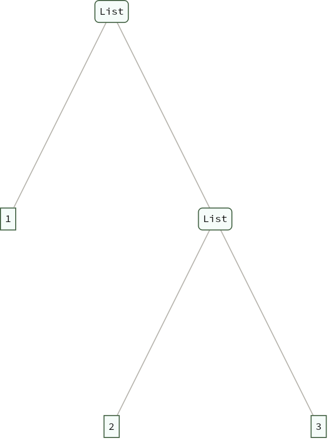
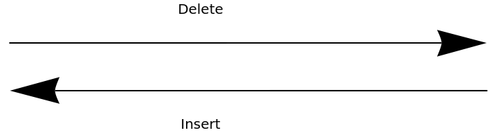
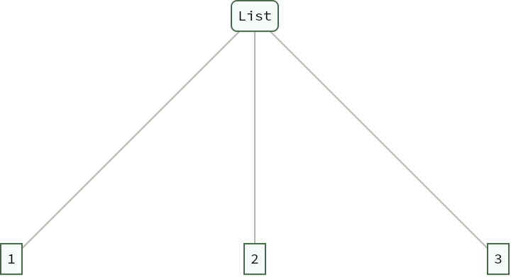
Before we calculate the edit distance we also have to consider the cost of inserting, removing and substituting a node. For this project, I have chosen all of these costs to be 1, however, any cost function, either constant or node specific, can be used.

Tree edit distance algorithms

The algorithms I have chosen to implement in this project are the ones described in Tai 1979, Zhang et al, 1989. Both are dynamic programing algorithms.

Tai’s algorithm

For Tai’s approach, the trees are traversed in a top down fashion and the distance between the smaller trees are calculated before the entire trees. We give an implementation of Tai's algorithm in Mathematica.

Zhang and Sasha algorithm

For Zhang’s method, we decompose both the trees into smaller and smaller subforests and calculate the edit distance between these subforests before calculating the total edit distance. The tree is traversed in a post order manner. This results in better space and time complexity compared to Tai’s algorithm. We give an implementation of Zhang's algorithm in Mathematica.

Examples

Example 1

To demonstrate the algorithm, we create two slightly different system of equations and calculate their distance as trees.

In[]:=

eqn1=-3c+4

0;eqn2=

1;Row[{te1=ExpressionTree[eqn1,ImageSize->Small],te2=ExpressionTree[eqn2,ImageSize->Small]},Spacer[36]]

Out[]=

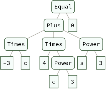
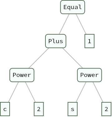
We can calculate the edit distance between the two trees:

In[]:=

TreeEditDistance[te1,te2]

Out[]=

Example 2

We create and import two Mathematica notebooks as trees .

In[]:=

nb1=CreateDocument[{TextCell["Heading","Section"],TextCell["Subsection","Subsection"],TextCell["Some text"],TextCell["Heading 2","Section"],TextCell["Subsection","Subsection"],TextCell["abcd"],TextCell["Subsection 2","Subsection"],TextCell["defg"]}];nb2=CreateDocument[{TextCell["Heading 1","Section"],TextCell["Some text"],TextCell["Heading 2","Section"],TextCell["Subsection","Subsection"],TextCell["See spot run"],TextCell["Subsection 2","Subsection"],TextCell["run spot run"]}];Row[{t1=ExpressionTree[NotebookImport[nb1,_,"FlattenCellGroups"->False],ImageSize->Medium],t2=ExpressionTree[NotebookImport[nb2,_,"FlattenCellGroups"->False],ImageSize->Medium]},Spacer[36]]

Out[]=

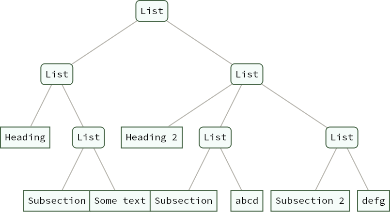
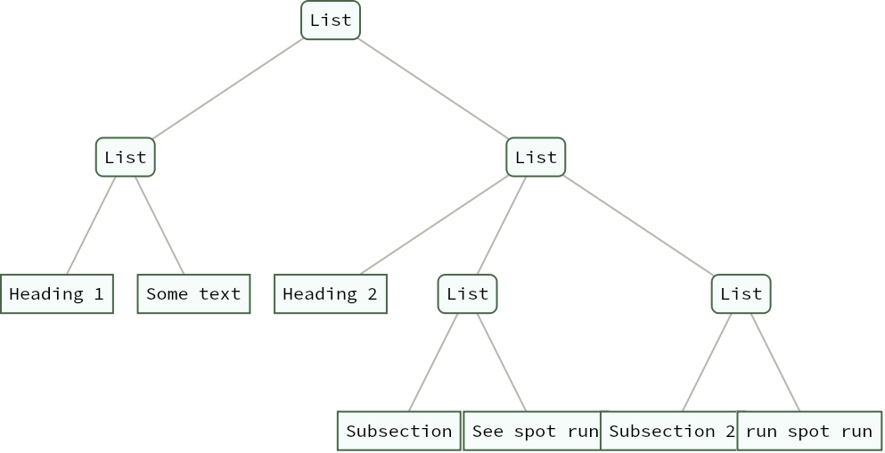
Then compute the edit distance between the two trees.

In[]:=

TreeEditDistance[t1,t2]

Out[]=

Minimal cost sequence of operations

We can also retrieve one of the minimal cost sequences of operations for converting one tree to another. We modify Zhang's code and show it.

For the two notebook trees shown above, the operations are as below:

In[]:=

{d,op}=TreeEditDistanceOp[t1,t2]

Out[]=

{5,{{Delete,1},{Substitute,2,1},{Match,3,2},{Match,4,3},{Delete,5},{Match,6,4},{Match,7,5},{Substitute,8,6},{Match,9,7},{Match,10,8},{Substitute,11,9},{Match,12,10},{Match,13,11},{Match,14,12}}}

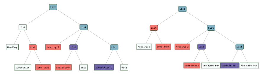
The number followed by Delete is the post order traversal position of the node of t1 to be deleted. Similarly, the numbers followed by Substitute and Match denote the post order traversal of t1 and t2 respectively. Note that these are operations on single nodes and not operations on the subtrees rooted at the nodes.

Based on these operations, we can show the matching parts of the two trees by highlighting them in different colors.

In[]:=

ShowMatch[t1,t2,op]

Out[]=

Future scope and Issues

Given the minimal sequence of operations, the goal is to be able to come up with a set of Mathematica tree operations that converts one tree to another. Unfortunately, this is not straightforward as the Insert operations given by the algorithms does not specify where in the first tree we should insert a certain node of the second tree. We demonstrate this problem below. The number followed by Insert operations denotes the post order traversal position of the node of the second tree to be inserted.

In[]:=

Rowt5=ExpressionTree[{1,2,3}],t6=ExpressionTree

,Spacer[36]TreeEditDistanceOp[t5,t6]

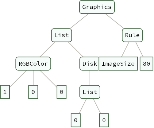
Out[]=

{11,{{Match,1,1},{Substitute,2,2},{Substitute,3,3},{Insert,4},{Insert,5},{Insert,6},{Insert,7},{Insert,8},{Match,4,9},{Insert,10},{Insert,11},{Insert,12},{Insert,13}}}

One possible workaround for this problem is to implement a similar tree transformation operation specified in Chawathe et al(https://doi.org/10.1145/235968.233366 ), using our minimal cost mapping. This will result in a minimal cost sequence of operations assuming that the cost of moving a subtree from one node to another node of the same parent tree is zero.

Definitions