Wolfram Cloud Document

ORIGINAL PRESENTATION: Alexander Kuznetsov, The coverage path planning problem with constraints on the path length and time. IMMOD-2023 conference, Kazan, Russia (18-20 October 2023). http://simulation.su/static/ru-immod-2023.html

The system under study consists of an agent - an UAV or a ground robot that monitors a given domain, and a mobile platform with which the agent has radio communication and to which the agent can return to recharge, receive or load the payload. We further study the following coverage path planning problem. A robot with limited battery power and a given viewing radius must cover a given domain. If the entire domain cannot be covered in one battery charge, then the robot divides the domain into sub-domain and returns to the starting point on the boundary of the domain to recharge before covering the next sub-area. If the entire domain cannot be covered in this way, then the robot minimally moves the starting point after covering as much of the domain as possible. A coverage path inside each sub-domain are constructed with the Concorde solver.

1
. Statement of the Problem

In the article, we will discuss the constrained version of the well-known coverage path planning problem [1-3].
Consider a bounded domain

D⊆



with a closed polygonal boundary ∂D. Further, we will refer to such a domain as a polygon and denote a set of such domains as . An agent ag should cover D with pairwise nonintersecting rectangles of a size a×b in a minimal possible time starting from a point

)∈∂D

. The agent ag has energy E to move along a path in the time T, i.e. a path of an agent moving with a constant speed v can have a length l=v T>0 only. After that, it must return to the point

. If D can’t be covered in this manner, we can change the starting point

to points

,...

∈∂D

. If D can’t be covered ever in this case, we can choose a starting point inside D.

The agent should delay at the points of interest

J={

,…,

}⊂D

.

There are two path planning options. In the first option, all information about the area is known in advance, the optimal path is calculated in advance, and the agent has a list of coordinates along which he must move. In the second option, the agent calculates the optimal path directly when passing through a domain, and changes in the state of a domain are possible. We will further assume the first option, which should always be considered, even if we use the second one, if only to check the quality of the heuristics. In the case of reactive route planning, the agent’s energy costs should be taken into account when calculating the optimal path.

An optimal route can be pre-calculated, in this case, energy spending on route planning is zero. Otherwise, the agent’s energy decrease on the amount E' at each act of planning and the maximal time of agent’s work is also decreased on the amount T'. Moreover, the domain D and the set J can change over time, and the pre-calculated path can turn suboptimal.

Additionally, an agent also has a communication range r and can’t move from the point

on a distance more than r.

When the aforementioned goal can’t be achieved, the agent can change the position of the start point.

We will consider the following possible events:

◼

Domain configuration change.

◼

Covering rectangle change.

◼

An agent's speed change.

◼

An agent's maximal path's length changes (due to the changes in wind direction or temperature).

◼

POI change.

We will consider the following transformations of the domain:

◼

Rotation

:

of the domain D on the angle α.

◼

Discretization

O,a,b

:RF

, i.e. building the grid of points

O+(na,mb),(n,m)∈



with the origin O. Here

RF⊂



is the set of all finite subsets of



. The rectangles of the size a×b with centres in point of the grid should cover the whole D.

◼

Split

p,β







the set (a domain D or a grid G) with a line starting from the point p and with a direction vector (cos α, sin α)

p,β

(D)=(x,y)∈Ddet

cosα	sinα
x- x 0	y- y 0

<0

◼

Skew







the set (a domain D or a grid G). It is a linear fractional transform defined by its homography matrix. This transform corresponds to the tilted position of an agent’s camera.

◼

Coverage C(D, G) of the domain D with rectangles centred in the points of the grid G.

Also, let L(G) be a solution of the travelling salesman problem for the grid G. The length function for this solution and weights for the TSP should be constructed taking into account the weights of points of interest.

To solve the problem, we should gradually split the domain into subdomains, where the aforementioned problem is feasible. The algorithm, in brief, should be as follows:

0. Set Remain=∅.

1. The domain D discretized to the grid

O,a,b

(

, where an angle α is such as

O,a,b

(

D)min

2. Solve the TSP for the grid G and search for the path L(G) subject to length(L(G))≤l.

3. If the problem is infeasible, we can choose steps 3.1 or 3.2, else go to step 4.2.

3.1. Split D and put

D'=

,β

(

, set

O,a,b

(

D')

, Remain = D∖ C(D',G). The β for the split domain

,β

(

should maximize the path L(G) subject to length(L(G))≤ l. Set D=D'.

4.1. Add (D, G, L(G)) to the Parts.

5.1. If Remain ≠ ∅, set G=Remain and go to step 2, else go to step 6.

3.2. Split the grid and put

G'=

,β

(

, set Remain = G∖ G'. The β for the split grid

,β

(

should maximize the path L(G) subject to length(L(G))≤ l. Set G=G'.

4.2. Add (D, G, L(G)) to the Parts.

5.2. If Remain ≠ ∅, set G=Remain and go to step 2, else go to step 6.

6. End.

Option 3.1 is suitable if the domain or the size of covering rectangles (i.e. if the agent rises or descends) can change in the process of monitoring. In this case, the next part of the domain can have a new grid with new size. Option 3.2 is more efficient computationally.

2. Generation of Random Domains

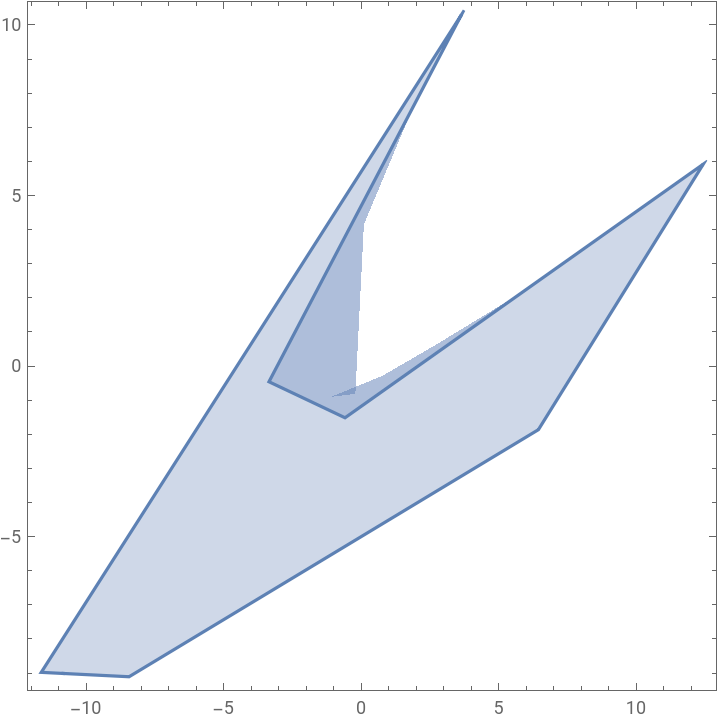
We will generate random Polygons as well as some other Domains of given area to test our Algorithms.

In[]:=

domainArea=100;

In[]:=

numberOfVertices=7;randomPolygon=RandomPolygon[numberOfVertices];scaleFactor=Sqrt[domainArea/Area[randomPolygon]];testDomain=RegionResize[randomPolygon,Scaled[scaleFactor]];

regionCentre=RegionCentroid[testDomain];

Default domain :

In[]:=

testDomain=Polygon[{{-11.632076767834924`,-8.979774293801224`},{-8.43847793369504`,-9.108207367921024`},{-3.3505065840563475`,-0.45964688456622227`},{-0.5844655253045019`,-1.5155266855993865`},{3.648556577631304`,10.299187165197484`},{6.449035996979013`,-1.864136488502833`},{12.44198812650156`,5.917833226657951`}},{1,2,6,7,4,3,5}];

In[]:=

RegionPlot[testDomain]

Out[]=

3. Building Grids

Set the Grid Cell size [4]. The actual value of these parameters depends on an agent’s height and an agent’s camera FOV.

In[]:=

visionRectX=1;visionRectY=1;

Let us construct the Grid.

The discretization transform

O,a,b

(we can also skew the grid):

In[]:=

discretize[testDomain_,precision_:.01]:=Module[{gridorigin,gridspace,cc},gridorigin=Floor[{Min[RegionBounds[testDomain][[1]]],Min[RegionBounds[testDomain][[2]]]}];gridspace={visionRectX,visionRectY};cc=N[Union[(({Round[#[[1]],gridspace[[1]]],Round[#[[2]],gridspace[[2]]]}+gridorigin+gridspace/2)&@(#-gridorigin-gridspace/2))&/@Select[MeshCoordinates[DiscretizeRegion[testDomain,MaxCellMeasureprecision]],Mod[#[[1]],visionRectX]≠0&&Mod[#[[2]],visionRectY]≠0&]]];{cc,gridspace,gridorigin}]

Here, we slightly improve the algorithm from [4] (see Appendix B).

In[]:=

testDomainCheck=testDomain;{cc,gridspace,gridorigin}=discretize[testDomainCheck];startccLength=Length[cc];cc1=cc;

We can rotate the Polygon for the best fit in a Grid.

The minimal rotation step can be defined as

-1

tan

visionRectY

regionXRange

2visionRectX

-1

tan

2visionRectXvisionRectY

regionXRange

In[]:=

ArcTan[N[(2*visionRectX*visionRectY)/regionXRange]]

Out[]=

0.073939

In[]:=

regionBounds=RegionBounds[testDomain];

In[]:=

regionCentre={regionBounds[[1,1]]+Abs[regionBounds[[1,2]]-regionBounds[[1,1]]]/2,regionBounds[[2,1]]+Abs[regionBounds[[2,2]]-regionBounds[[2,1]]]/2};

The rotation transform

with an optimized α:

In[]:=

rotate[testDomain_,angleStep_:0.1]:=MinimalBy[Map[{#,discretize[TransformedRegion[testDomain,RotationTransform[#]]],TransformedRegion[testDomain,RotationTransform[#]]}&,Range[0,2Pi,angleStep]],Length[#[[2,1]]&]];

We obtain that the Polygon should be rotated on

In[]:=

rotate[testDomain][[1,1]]

Out[]=

Rotate the Polygon and calculate bounds :

In[]:=

{α,{cc,gridspace,gridorigin},testDomain}=rotate[testDomain][[1]];regionBounds=RegionBounds[testDomain];regionYRange=Ceiling[Abs[regionBounds[[2,2]]-regionBounds[[2,1]]]];regionXRange=Ceiling[Abs[regionBounds[[1,2]]-regionBounds[[1,1]]]];

In[]:=

regionMapConstruct=.regionMapConstruct[testDomain_,gridorigin_,gridspace_,regionXRange_,regionYRange_,cc_]:=RegionPlot[testDomain,PlotRangeAll,Prolog{{FaceForm[Blue],Rectangle[#-gridspace/2,#+gridspace/2]&/@cc},Line[{gridorigin+{#,0},gridorigin+{#,regionYRange+2}}]&/@Range[0,regionXRange,gridspace[[1]]],Line[{gridorigin+{0,#},gridorigin+{regionXRange+2,#}}]&/@Range[0,regionYRange,gridspace[[2]]]},AspectRatioAutomatic];

Plot Centers of the Cells

Our rotation procedure reduces the size of the Polygon’s Greed on:

We can also skew the region, i.e. we can tilt an agent’s camera in such way that the domain will be covered with a reduced number of distorted frames [5-7]. It can be useful for reducing computational complexity of coverage algorithms.

Let us describe the transformation matrix. Here, we use only a perspective without any rotation or translation transforms. Obviously, when the agent moves, the transformation matrix must change.

Define the inverse transform:

After inverse transformation, we obtain the skewed coverage of the domain.

The grid was significantly reduced in this way:

We should change the transformation matrix when move to preserve the form of the skewed domain:

Further, we can discretize various regions, not only polygonal ones [4], see Appendix B.

4. Calculating the shortest path in one Domain.

We will use the Wolfram Mathematica function FindShortestTour[...]. When possible, it uses the Concorde program under the hood. The possible methods are “AllTours”, “CCA”, “Greedy”, “GreedyCycle”, “IntegerLinearProgramming”, “OrOpt”, “OrZweig”, “RemoveCrossings”, “SpaceFillingCurve”, “SimulatedAnnealing”, or “TwoOpt”.
https://community.wolfram.com/groups/-/m/t/478978

The Concorde program is available at the site
https://www.math.uwaterloo.ca/tsp/concorde.html

In the case of a rectangular grid, the longest path problem has the linear-time algorithm of solution [8-9].

Smoother variant with splines :

5. Splitting the Domain

In this Notebook, we solve the CCP problem in the case when UAV can cover only the part of the Domain without recharge. So, we should split the Domain.
Let us take the arbitrary point:

For the further algorithm, we will write the Polygon in the special representation with ordered vertices:

The agent' s start position is the closest to the agentStartPosition point into the Polygon boundary.

The Polygon will be split on pieces with a straight line:

An example:

6. Calculating an optimal Path in Subdomains

6.1. What is the maximal area for the given maximal path for CCP?

Let the maximal possible path of the Agent be

The worst case when the Agent crosses Cells diagonally:

In the common case, we can choose

Define the Polygons of the Grid

6.2. The pathfinding procedure

This function tries to split the Domain onto the pieces with area which is the closest to maxArea.

Let us find the nearest to the agent’s start point cell:

The first option (we split the grid directly):

The second option (we split the domain):

If the resulting Path is greater or lesser than the maximal possible one, we should reduce or increase the area of the Domain' s piece. The Procedure can be optimized for convex Polygons (see Section 7).

After that, we should find intersections of the partial Domain with Grid.

The area of the partial Domain:

The calculated shortest path:

The difference between the calculated shortest path and the maximal possible path:

Let us display the obtained partial Domain and the shortest path on it:

The agent’s start position is marked by the yellow rectangle.

Let us find the remaining part of the Domain

Finally, we can depict the remaining Domain and the optimal Path on it.

The agent’s start point can be not included in the new grid:

So, it is necessary to append the start point:

The length of the path into the remaining region:

6.3. Automation of Polygon Division

This routine automatizes the Domain splitting process (see also [10, 11]). We can also apply the rotation transform before the discretization of the next sub-domain to reduce the number of cells as in Section 2 and then apply the inverse rotation transform to the cells obtained.

Let us depict the result of the splitting and pathfinding process:

7. The Case of a Convex Polygon

In the case of a convex polygon, we can split it in a particular way, changing the angle of a splitting line not from 0 to 2 π but in a lesser span. This can be useful for optimisation purposes.

We will consider two cases: the starting point is at the vertex of the polygon and the starting point is on the edge of the polygon. Let us take a two Points on the Polygon’s Boundary.

This Function determines if a Point is a Polygon’s Vertex (in this cases the Function returns “True” in the second component) and also returns the two nearest distinct vertices to this given Point.

Let us determine which side on the right and which side on the left

Which is above and which is below the Point.

Let us determine an Angle at the Point.

Let us determine if the Polygon is under the Line or above the Line:

We can summarize the search of the cutting angles in the following manner:

Let us consider the second case:

For a convex polygon, it is necessary to continue cutting off parts until the sign of the difference between the resulting path and the maximum possible one changes.

8. Changing the Start Position

Sometimes, it is not possible to split a Polygon into lesser Polygons such that an Agent can cover them from the single Position. It these cases, we should change the position. For practical Reasons, we should prefer to choose a new Position on the Polygon' s Boundary.

We have no splitting options.

We can change the start point. From the practical considerations, the new start position should be preferably on the domain’s boundary. The reason is that in agricultural applications agent shouldn’t cross the fields to avoid damage to valuable plants.

Also, we can triangulate [12] the Polygon into smaller Polygons with the Area’s size of maxArea.

We can use any of the following points on the polygon boundary as the agent’s start position.

We should choose as start positions points which are common vertices of the largest possible number of triangles:

Other start points can be found as the following:

Define order of start points

Introduce the special distance on the polygon’s boundary. This metric can be used for calculating the best order of changing of start points as well as in order to plan the energy costs for the base station.

Let us finally calculate the optimal order of the starting points. In the simplest case, we can simply go around the polygon clockwise (or counterclockwise).

In this case, we can cover a lot of triangles without changing a start point. But paths in the triangles can be suboptimal, and we can merge triangles to find more optimal paths.

What is the criterion for applying the triangulation process? For example, in an equilateral triangle, changing the starting point can be useless. We will suppose to triangulate the region if all its sides are longer than agentMaxPathLength/2.

9. Changing weights of some special Points

Sometimes, an Agent should make delay in some Points. In this case, TSP should have the special Metric.

It can be done by modifying the distance function (actually, by defining a weight matrix) and could be solved via standard solvers like Concorde.

If an Agent should make delay in these points only once or by a given number of times, the TSP transforms to a difficult Dynamic TSP problem. A Metric should have some Global Variables inside. In this case, we should use a custom solver. For example, we can use the Genetic Algorithm or Ant Colony Algorithm as described in [13, 14].

10. Computational Complexity of the Algorithm

We calculate the experimental data with the following cycle and store it in Appendix A.

Bibliography

1. Enric Galceran, Marc Carreras, A survey on coverage path planning for robotics, Robotics and Autonomous Systems, Volume 61, Issue 12, 2013, Pages 1258-1276, ISSN 0921-8890. https://doi.org/10.1016/j.robot.2013.09.004

2. Fevgas, G.; Lagkas, T.; Argyriou, V.; Sarigiannidis, P. Coverage Path Planning Methods Focusing on Energy Efficient and Cooperative Strategies for Unmanned Aerial Vehicles. Sensors 2022, 22, 1235. https://doi.org/10.3390/s22031235

3. Acevedo, Jose & Arrue, Begoña & Maza, Ivan & Ollero, Anibal. (2013). Distributed Approach for Coverage and Patrolling Missions with a Team of Heterogeneous Aerial Robots Under Communication Constraints. International Journal of Advanced Robotic Systems. 10. 1-13. 10.5772/52765. https://www.researchgate.net/publication/259667679_Distributed _Approach _for _Coverage _and _Patrolling _Missions _with _a _Team _of _Heterogeneous _Aerial _Robots _Under _Communication _Constraints

4. https://mathematica.stackexchange.com/questions/126346/how-to-quickly-find-all-grid-cells-covered-by-a-geometric-region

5. https://www.scratchapixel.com/lessons/3d-basic-rendering/perspective-and-orthographic-projection-matrix/opengl-perspective-projection-matrix.html

6. https://ogldev.org/www/tutorial12/tutorial12.html

7. https://en.wikipedia.org/wiki/Transformation_matrix

8. Fatemeh Keshavarz-Kohjerdi, Alireza Bagheri, Asghar Asgharian-Sardroud, A linear-time algorithm for the longest path problem in rectangular grid graphs, Discrete Applied Mathematics, Volume 160, Issue 3, 2012, Pages 210-217, ISSN 0166-218X. https://doi.org/10.1016/j.dam.2011.08.010.

9. https://stackoverflow.com/questions/22472732/polynomial-time-algorithm-for-travelling-salesman-in-a-grid

10. https://mathematica.stackexchange.com/questions/137957/extract-boundary-points-from-boundarymeshregion

11. https://mathematica.stackexchange.com/questions/226735/how-to-fill-in-interior-in-a-mesh-region

12. Weisstein, Eric W. "Triangulation." From MathWorld--A Wolfram Web Resource. https://mathworld.wolfram.com/Triangulation.html

13. Li, C., Yang, M., Kang, L. (2006). A New Approach to Solving Dynamic Traveling Salesman Problems. In: , et al. Simulated Evolution and Learning. SEAL 2006. Lecture Notes in Computer Science, vol 4247. Springer, Berlin, Heidelberg. https://doi.org/10.1007/11903697_ 31

14. Adam DeJans. Solving the Dynamic Travelling Salesman Problem (DTSP) via Ant Colony Optimization (June 2018) https://github.com/addejans/Dynamic-TSP

CITE THIS NOTEBOOK

The coverage path planning problem with constraints on the path length and time
by Alexander Kuznetsov
Wolfram Community, STAFF PICKS, August 23, 2023
https://community.wolfram.com/groups/-/m/t/2997003

1. Statement of the Problem

2. Generation of Random Domains

3. Building Grids

4. Calculating the shortest path in one Domain.

5. Splitting the Domain

6. Calculating an optimal Path in Subdomains

6.1. What is the maximal area for the given maximal path for CCP?

6.2. The pathfinding procedure

6.3. Automation of Polygon Division

7. The Case of a Convex Polygon

8. Changing the Start Position

9. Changing weights of some special Points

10. Computational Complexity of the Algorithm

Bibliography

CITE THIS NOTEBOOK

1
. Statement of the Problem