This code addresses the correlation of liquid–liquid equilibrium (LLE) data for a binary system using the Non-Random Two-Liquid (NRTL) thermodynamic model. Experimental tie-line data, comprising mole fractions in both phases (x_phaseI and x_phaseII) and their corresponding equilibrium temperatures, were used as the basis for parameter regression. The NRTL model activity coefficients were implemented as a function of the binary interaction parameters A12, A21, B12, and B21, with the non-randomness parameter α fixed at 0.20. A modified Gibbs free energy of mixing formulation (gmixRT) was defined to allow the phase equilibrium calculations.
To determine phase compositions consistent with thermodynamic equilibrium at each experimental temperature, a common tangent line construction was implemented. For each tie-line, the slopes of the Gibbs energy curve were computed via automatic differentiation at trial compositions xa and xb, and a system of two nonlinear equations (equal slopes and equal tangent-line values) was solved numerically using FindRoot with a fixed initial guess.
The core objective function was constructed as the sum of squared deviations between calculated and experimental compositions in both liquid phases across all tie-lines. Rather than relying on a local gradient-based solver — which can be sensitive to initial guesses and prone to converging on local minima — the parameters A12, A21, B12, and B21 were estimated using Particle Swarm Optimization (PSO), a population-based global meta-heuristic. The custom PSO implementation used 30 particles, 100 iterations, inertia weight decay equal to 0.72984, and cognitive/social coefficients of 1.42, with velocity clamping and boundary clipping to maintain feasible search space. The optimizer converged to a fitness value of 4.48 × 10⁻⁴.
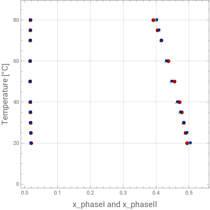
The PSO-derived parameter set was benchmarked against literature-reported values for the same system (Ref. 2), which yielded a fitness value of 4.90 × 10⁻⁴ when evaluated under the identical objective function. This represents an improvement of roughly 9% in fit quality, indicating that the PSO approach identified a parameter combination that more accurately reproduces the experimental phase compositions (given in Ref. 1) than the previously published regression of Ref. 2. This improvement is further illustrated through a phase diagram comparing experimental, PSO-fitted, and literature-based tie-line predictions, as well as a convergence plot showing the PSO algorithm’s fitness trajectory rapidly decreasing and stabilizing below the literature benchmark within the first 20–30 iterations.
Experimental data from Ref.1
data2exp=;
NRTL Model
nrtlGex[x1_,tau12_,tau21_,alpha_]:=Module[{x2,G12,G21},x2=1-x1;G12=Exp[-alpha*tau12];G21=Exp[-alpha*tau21];x1*x2*(tau21*G21/(x1+x2*G21)+tau12*G12/(x2+x1*G12))]gmixRT[x1_,tau12_,tau21_,alpha_]:=Module[{x2},x2=1-x1;x1*Log[x1]+x2*Log[x2]+nrtlGex[x1,tau12,tau21,alpha]]
Common tangent
commonTangent[tau12_,tau21_,alpha_]:=Module[{ga,gb,slope,eq1,eq2,guess,sol,xa,xb},guess={0.005,0.5};ga=gmixRT[xa,tau12,tau21,alpha];gb=gmixRT[xb,tau12,tau21,alpha];slope=(gb-ga)/(xb-xa);eq1=D[gmixRT[x,tau12,tau21,alpha],x]/.x->xa;eq2=D[gmixRT[x,tau12,tau21,alpha],x]/.x->xb;sol=FindRoot[{eq1-slope==0,eq2-slope==0},{{xa,guess[[1]]},{xb,guess[[2]]}},MaxIterations->200,PrecisionGoal->8,AccuracyGoal->8];{xa,xb}/.sol]
Non-randomness parameter is fixed equal to 0.2
alpha=0.20;
PSO-parameters and problem dimension
SwarmDim=4;c1=1.42;c2=1.42;w=0.72984;
Upper and lower bounds
FitnessLB={-4.2,8.4,720,-1150};FitnessUB={-2.2,9.5,890,-950};
Fitness function
In[]:=
Fitness[{A12_,A21_,B12_,B21_}]:=Module[{tbl,tau12,tau21,fit,T},fit=0;Do[T=data2exp[[i]][[1]];tau12=A12+B12/T;tau21=A21+B21/T;tbl=commonTangent[tau12,tau21,alpha];fit=fit+(tbl[[1]]-data2exp[[i]][[2]])^2+(tbl[[2]]-data2exp[[i]][[3]])^2,{i,1,Length@data2exp}];fit]
Clip each column of a matrix against its own scalar bound
clipMatrix[mat_,lbv_,ubv_]:=Transpose[MapThread[Clip[#1,{#2,#3}]&,{Transpose[mat],lbv,ubv}]];clampMatrix[mat_,vmaxv_]:=Transpose[MapThread[Clip[#1,{-#2,#2}]&,{Transpose[mat],vmaxv}]];
PSO code
PSO code
PSO Optimizer
psoOptimize[lossFunc_,dim_,lb_,ub_,nParticles_:30,nIter_:100,wMax_:0.9,wMin_:0.4,c1_:1.42,c2_:1.42,vClampFrac_:0.2]:=Module[{particles,velocities,pbest,pbestScore,gbest,gbestScore,convergence={},r1,r2,scores,gbestIdx,vmax,wIter},vmax=vClampFrac*(ub-lb);particles=Transpose@Table[RandomReal[{lb[[i]],ub[[i]]},nParticles],{i,dim}];velocities=ConstantArray[0.,{nParticles,dim}];pbest=particles;pbestScore=lossFunc/@particles;gbestIdx=First@Ordering[pbestScore,1];gbestScore=pbestScore[[gbestIdx]];gbest=pbest[[gbestIdx]];Do[wIter=wMax-(wMax-wMin)*(t-1)/(nIter-1);r1=RandomReal[1,{nParticles,dim}];r2=RandomReal[1,{nParticles,dim}];velocities=wIter*velocities+c1*r1*(pbest-particles)+c2*r2*(ConstantArray[gbest,nParticles]-particles);velocities=clampMatrix[velocities,vmax];particles+=velocities;particles=clipMatrix[particles,lb,ub];scores=lossFunc/@particles;pbest=MapThread[If[#3<#2,#1,#4]&,{particles,pbestScore,scores,pbest}];pbestScore=MapThread[Min,{pbestScore,scores}];gbestIdx=First@Ordering[pbestScore,1];If[pbestScore[[gbestIdx]]<gbestScore,gbestScore=pbestScore[[gbestIdx]];gbest=pbest[[gbestIdx]];];AppendTo[convergence,gbestScore];If[t<10||Mod[t,10]==0,Print["PSO Iter ",t," Loss = ",gbestScore]];,{t,nIter}];{gbest,gbestScore,convergence}];
PSO run
result=psoOptimize[Fitness,SwarmDim,FitnessLB,FitnessUB,30,100];{gbest,gbestScore,convergence}=result;
PSO Iter 1 Loss = 0.000675645
PSO Iter 2 Loss = 0.000675645
PSO Iter 3 Loss = 0.000614191
PSO Iter 4 Loss = 0.000579516
PSO Iter 5 Loss = 0.000557193
PSO Iter 6 Loss = 0.000530044
PSO Iter 7 Loss = 0.000477723
PSO Iter 8 Loss = 0.000477723
PSO Iter 9 Loss = 0.00044824
PSO Iter 10 Loss = 0.00044824
PSO Iter 20 Loss = 0.00044824
PSO Iter 30 Loss = 0.000445373
PSO Iter 40 Loss = 0.000444696
PSO Iter 50 Loss = 0.000443016
PSO Iter 60 Loss = 0.000443016
PSO Iter 70 Loss = 0.000442933
PSO Iter 80 Loss = 0.000442877
PSO Iter 90 Loss = 0.00044283
PSO Iter 100 Loss = 0.000442773
PSO-derived values for A12, A21, B12 and B21 and the corresponding value of the fitness function ≈ 4.48 10^-4
In[]:=
gbestgbestScore
Out[]=
{-3.72016,8.47562,790.844,-989.439}
Out[]=
0.000442773
Literature values for A12, A21, B12 and B21 (see Ref. 2) and the corresponding value of the fitness function ≈ 4.90 10^-4
In[]:=
sollit={-3.74,8.69,795,-1057}Fitness[sollit]
Out[]=
{-3.74,8.69,795,-1057}
Out[]=
0.00049084
Calculated LLE data versus experimental data from Ref. 1
mylle[{A12_,A21_,B12_,B21_}]:=Module[{tbl,tau12,tau21,fit,T},tbl={};Do[T=data2exp[[i]][[1]];tau12=A12+B12/T;tau21=A21+B21/T;pt=commonTangent[tau12,tau21,alpha];AppendTo[tbl,pt],{i,1,Length@data2exp}];tbl]
In[]:=
mydata=mylle[gbest]
Out[]=
{{0.0184585,0.504384},{0.018275,0.493898},{0.0181065,0.483816},{0.0179515,0.474123},{0.0178089,0.464803},{0.0175562,0.447222},{0.0173411,0.430953},{0.0171577,0.415882},{0.0170763,0.408762},{0.0170011,0.401902}}
In[]:=
mydata2=mylle[sollit]
Out[]=
{{0.0189967,0.501158},{0.0187221,0.490917},{0.0184674,0.481075},{0.0182307,0.471615},{0.0180104,0.462524},{0.0176132,0.445384},{0.0172659,0.429535},{0.0169608,0.414864},{0.016822,0.407937},{0.0166914,0.401266}}
p2=ListPlot{Transpose@{data2exp[[All,2]],data2exp[[All,1]]-273.15},Transpose@{data2exp[[All,3]],data2exp[[All,1]]-273.15}},;myp=ListPlot{Transpose@{mydata[[All,1]],data2exp[[All,1]]-273.15},Transpose@{mydata[[All,2]],data2exp[[All,1]]-273.15}},;refp=ListPlot{Transpose@{mydata2[[All,1]],data2exp[[All,1]]-273.15},Transpose@{mydata2[[All,2]],data2exp[[All,1]]-273.15}},;Showp2,myp,refp,PlotRange->{{0,0.55},{0,85}},
Out[]=
PSO Convergence Plot - PSO result is better than the literature values reported in Ref. 2 (i.e., it yields a lower fitness function value)
References
References
[1] Andrzej Maczynski, David G. Shaw, Marian Goral, Barbara Wisniewska-Goclowska, IUPAC-NIST Solubility Data Series. 82. Alcohols with Water—Revised and Updated: Part 1. C4 Alcohols with Water. J. Phys. Chem. Ref. Data 1, March 2007; 36 (1): pp. 59–132.
[2] Danielle L. de Klerk and Cara E. Schwarz, Simplified Approach to the Parameterization of the NRTL Model for Partially Miscible Binary Systems: Tττ LLE Methodology, Industrial & Engineering Chemistry Research, 2023 62 (4), pp. 2021-2035. DOI: 10.1021/acs.iecr.2c03953
CITE THIS NOTEBOOK
CITE THIS NOTEBOOK
PSO for NRTL model parameter estimation in liquid–liquid equilibrium (LLE) binary systems
by Housam Binous
Wolfram Community, STAFF PICKS, July 1, 2026
https://community.wolfram.com/groups/-/m/t/3742066
by Housam Binous
Wolfram Community, STAFF PICKS, July 1, 2026
https://community.wolfram.com/groups/-/m/t/3742066