
Introduction
Introduction
Wolfram Models & Emergent Geometry
Wolfram Models & Emergent Geometry
The class of models introduced with the Wolfram Physics Project are, at their most fundamental level, abstract rewriting rules for transforming different relations in a subhypergraph. There really is no a priori definition of space, time, matter, or geometry. However, as the transformation rules are applied with an increasing number of steps, sundry properties of fundamental physics emerge as a sort of natural consequence of the graph’s evolution. One such property that has been found to emerge and is essential for the characterization of the laws of physics using this model, is the notion of geometry. After a large number of steps in the evolution of the graph, what appears to be a rendition of space emerges and can be studied. One of the most relevant properties that can be of great use in its applications to the study of physics is the notion of dimension.
For any flat, continuous space, one can trivially define dimension and think of it in terms of the number of coordinates necessary to describe any point in that space. But, in the study of Wolfram Model evolution systems, it becomes necessary to find different ways of characterizing dimension. One such way, that is explained in detail in the Physics Project’s Technical Introduction[1], is to define a quantity(X) which is essentially the volume of a ball of radius starting from a center point located in the graph at position , i.e. the number of points near that can be reached (starting from ) by going a distance no larger than . By then taking log differences of (X), one can make an estimate of the approximate dimensionality of the graph.
The important takeaway from this is that, even though there is no definition in the model of what dimension is or should be, as the graphs are evolved with a certain transformation rule, what can be definitively characterized as dimension emerges and can be studied. Yet another way of estimating the dimension of the graph is by looking at the causal graph of the evolution of the system. From the evolution of a Wolfram Model, one can construct a causal graph that represents the different updating events that occur in the evolution and their causal dependence on one another (i.e. “how much of the output of one event forms the input of another event?” and vice versa).
For any flat, continuous space, one can trivially define dimension and think of it in terms of the number of coordinates necessary to describe any point in that space. But, in the study of Wolfram Model evolution systems, it becomes necessary to find different ways of characterizing dimension. One such way, that is explained in detail in the Physics Project’s Technical Introduction[1], is to define a quantity
V
r
r
X
X
X
r
V
r
The important takeaway from this is that, even though there is no definition in the model of what dimension is or should be, as the graphs are evolved with a certain transformation rule, what can be definitively characterized as dimension emerges and can be studied. Yet another way of estimating the dimension of the graph is by looking at the causal graph of the evolution of the system. From the evolution of a Wolfram Model, one can construct a causal graph that represents the different updating events that occur in the evolution and their causal dependence on one another (i.e. “how much of the output of one event forms the input of another event?” and vice versa).
Causal Sets, and Dimension Estimation
Causal Sets, and Dimension Estimation
Causal Set Theory[2] is an approach to quantum gravity primarily developed by R. Sorkin, L. Bombelli, J. Lee, and D. Meyer in the late 1980s and in which it is stated that spacetime is not a continuum but rather a collection of discrete points endowed with a partial order relation of the form x ≺ y, i.e. “x is to the past of y.” These partial order relations are acyclic(antisymmetric), transitive, and locally finite. In the context of this theory, there is a method for estimating the dimension of the manifold into which the causal set embeds, known as the Myrheim-Meyer dimension estimator algorithm[3]. This algorithm involves choosing two points in the causal set which determine what is known as an Alexandrov Interval (or causal diamond), which is simply the intersection of the future of an event with the past of an event . One can then take a suitable ratio between the number of causal relations in that interval (i.e. pairs of the form x ≺ y) as well as the number of points on that same interval. This specifically defined ratio is then a function solely of the dimensionality of the manifold, therefore providing a way to estimate this dimension.
As amply detailed by J. Gorard[4], one can draw several relations between the Wolfram Model and the causal networks constructed with them and the properties of the causal sets. Specifically, the transitive reduction of the causal networks forms the Hasse Diagram of the causal partial order, i.e. the transitive reduction of the causal network satisfies the axioms of the causal set. We can therefore utilize methods such as the Myrheim-Meyer dimension estimator and apply them to characterize different properties (in this case the approximate dimension) of Wolfram Model evolution systems.
p
q
d
As amply detailed by J. Gorard[4], one can draw several relations between the Wolfram Model and the causal networks constructed with them and the properties of the causal sets. Specifically, the transitive reduction of the causal networks forms the Hasse Diagram of the causal partial order, i.e. the transitive reduction of the causal network satisfies the axioms of the causal set. We can therefore utilize methods such as the Myrheim-Meyer dimension estimator and apply them to characterize different properties (in this case the approximate dimension) of Wolfram Model evolution systems.
Perturbations in dimension
Perturbations in dimension
In classical General Relativity, there exists the well-defined notion of perturbations in the curvature of spacetime, and how these curvature perturbations can ripple through the fabric of spacetime, giving rise to the phenomena of gravitational radiation. In that regard, since the overall objective of the Wolfram Model is to not only describe the fundamental laws of the universe, but also find different phenomena not already encountered in the current worldview of physics, one important question that arises from the study of dimension in the Wolfram Model, is how that dimension can be affected or perturbed in the evolution of a graph. What effects can a perturbation in the local dimension of a subgraph have in the overall approximate dimensionality of the graph? And how can that perturbation spread throughout the graph? The goal of this project is to analyze the effects of such perturbations. In order to achieve this, we must first establish a reliable mechanism via which we can characterize the dimension of a graph, and how that dimension changes in different regions of the overall structure. Thus will be the topic of the following sections.
Characterizing Dimension in Wolfram Model Systems
Characterizing Dimension in Wolfram Model Systems
Measuring Dimension Locally
Measuring Dimension Locally
As explained above, one can approximate the dimension a specific region in a causal set by making use of the Myrheim-Meyer dimension estimation formula:
,
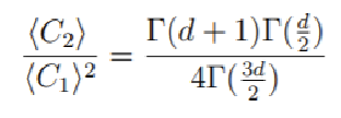
Myrheim-Meyer formula for dimension estimation
where is the average number of causal relations in the interval and is the average number of points in that same interval. The right-hand side (RHS) is a monotonic function of the dimension of the manifold. With this, we were able to construct a function that takes as input a causal graph as well as a specification of a start and end vertex in said graph (which determine the Alexandrov interval or causal diamond to be used for estimation):
C
2
C
1
d
Function to estimate the dimension of a causal diamond using the Myrheim-Meyer formula
CausalDiamondDimensionEstimator[causalGraph_Graph,startVertex_Integer,endVertex_Integer]:=Module[{causalDiamond,d}, causalDiamond = TransitiveClosureGraph[Subgraph[causalGraph, Intersection[VertexInComponent[causalGraph, endVertex],VertexOutComponent[causalGraph, startVertex]]]]; If[EmptyGraphQ[causalDiamond],Infinity, Replace[d, FindRoot[{ EdgeCount[causalDiamond]/((VertexCount[causalDiamond])^2)(Gamma[d+1]*Gamma[d/2])/(4Gamma[3d/2])},{d,1,0,Infinity}]]]]
Wherein we are taking the transitive closure of the provided causal graph, which corresponds to the causal set of the evolution, i.e. the set of all relations x ≺ y. Then, we are solving for the dimension on the RHS of the Myrheim-Meyer estimation formula, using EdgeCount and VertexCount to determine the ratio on the left-hand side.
d
Estimating Dimension from a Transformation Rule
Estimating Dimension from a Transformation Rule
In order to have a way of determining the effect of a dimension perturbation in the evolution of a graph, one not only needs a way of measuring dimension locally, one also needs to determine which initial conditions are to be used a a starting point for the rule and, not trivially, which transformation rule is to be applied. The rule to be used must have the condition that it preserves the approximate dimension of the initial state with successive generations. If we want to perturb the dimension and see how the perturbation spreads, it cannot also be the case that the rule itself will further perturb the dimension, as that will result in not very useful results.
For that end, we constructed two functions, FindEndEvents and ResultingDimensionOfRule. The former is a function which, given a causal graph and a specific vertex in it, will return a list of all the “ending events,” i.e. all events with out-degree of 0 that lie in the out-component of the given vertex. The latter will take as input a Wolfram Model transformation rule, a list of initial conditions, a number of generations, and a sample size. It then applies the given rule to the initial conditions for the specified number of generations, and proceeds to estimate the dimension of the graph by applying the CausalDiamondDimensionEstimator function, starting from a random sample of the starting events (i.e. those with in-degree of 0). We thus have a way of determining the approximate dimensionality of the resulting structure that a particular rule produces after some number of generations. The definitions of the functions are the following:
For that end, we constructed two functions, FindEndEvents and ResultingDimensionOfRule. The former is a function which, given a causal graph and a specific vertex in it, will return a list of all the “ending events,” i.e. all events with out-degree of 0 that lie in the out-component of the given vertex. The latter will take as input a Wolfram Model transformation rule, a list of initial conditions, a number of generations, and a sample size. It then applies the given rule to the initial conditions for the specified number of generations, and proceeds to estimate the dimension of the graph by applying the CausalDiamondDimensionEstimator function, starting from a random sample of the starting events (i.e. those with in-degree of 0). We thus have a way of determining the approximate dimensionality of the resulting structure that a particular rule produces after some number of generations. The definitions of the functions are the following:
Functions to find the ending events of a causal diamond and to estimate the dimension of the structure resulting from a Wolfram Model rule
FindEndEvents[causalGraph_Graph, startEvent_Integer]:= Module[{}, Select[Drop[VertexOutComponent[causalGraph, startEvent], 1], VertexOutDegree[causalGraph, #] 0 &]]ResultingDimensionOfRule[transformationRule_Rule, initialConditions_List, generations_Integer, sampleEvents_Integer] := Module[{object, causalGraph, startEvents}, object=WolframModel[transformationRule,initialConditions,generations]; causalGraph=object["CausalGraph"]; startEvents=Position[object["EventGenerations"], 1]; If[Length[startEvents] ≠ 0, MeanAround[Flatten[DeleteCases[Map[With[{endEvents=FindEndEvents[causalGraph, #]}, If[Length[endEvents] ≠ 0, CausalDiamondDimensionEstimator[causalGraph, #, RandomChoice[endEvents]]]]&,RandomSample[startEvents, sampleEvents],{2}], Null, All]]], Failure["RuleTerminated",<| "MessageTemplate""Rule `Rule` did not produce enough generations", "MessageParameters"<|"Rule"transformationRule|>|>]]]
Where we have made use of the SetReplace library originally developed by Max Piskunov. We can test these functions by generating a random wolfram model with signature , starting from a simple cycle graph:
2
2
3
2
ResultingDimensionOfRule[BlockRandom[ ResourceFunction["RandomWolframModel"][{{2,2}} {{3,2}}], List @@@ EdgeList[CycleGraph[50]], 10, 5], RandomSeeding 0]
Out[]=
2.
An interesting result since it means the random rule has resulted in a 1 + 1-dimensional causal network, i.e. the rule has actually preserved the dimensionality of the cycle graph.
Initial Conditions
Initial Conditions
For the purposes of this project, we opted to use a 2-dimensional toroidal structure as the initial conditions which we would then evolve by applying the transformation rules. Obtaining such a structure would be easier than having to generate one using a Wolfram Model rule starting from a single expression. We can obtain this torus by randomly generating a set of coordinates, shifting half of them, and finally merging both sets (removing any duplicate points). That is what the following code is executing:
BlockRandom[With[ coordinates = RandomReal[1,{1500,2}], edgeMaxDistance = 0.06, torus = IndexGraph[GraphUnion[ NearestNeighborGraph[coordinates,{All,edgeMaxDistance}], VertexReplace[NearestNeighborGraph[Map[If[#<0.5,#+1,#]&,coordinates,{2}],{All,edgeMaxDistance}], {x_,y_}(If[#>1,#-1,#]&/@{x,y})]]]], RandomSeeding 0]
Out[]=
Graph


From which we obtain:
In[]:=
GraphPlot[torus]
Out[]=
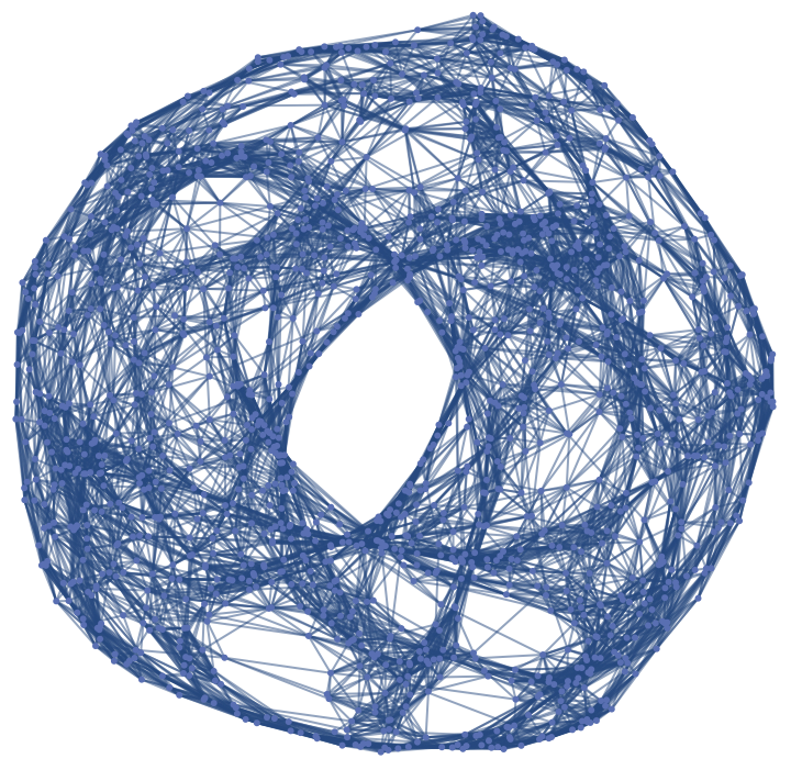
Torus created as the initial condition for the analysis of transformation rules
Finding a Rule that Preserves Dimension
Finding a Rule that Preserves Dimension
We have now established a mechanism for finding the resulting dimension of the structure produced by a given transformation rule, and we have constructed the initial conditions for the application of these rules. We are thus in a position to start searching for rules that are able to preserve the dimensionality of the initial condition, i.e. the torus constructed. Doing a completely-extensive search requires an enormous amount of computational power. We were still able to do a fairly comprehensive search, first starting with a simpler case of using a cycle graph as the initial condition. We were thus looking for rules that would create a 1 + 1-dimensional causal graph. We were able to find several of them, among which were:
{{1,2}, {2,3}} {{1,1}, {4,3}}{{1,2}, {2,3}} {{2,1}, {3,4}}{{1,2}, {2,3}} {{4,2}, {4,3}}{{1,2}, {2,3}} {{2,1}, {4,3}} |
{{1,2}, {2,3}} {{3,1}, {3,1}}{{1,2}, {2,3}} {{2,1}, {2,1}}{{1,2}, {2,3}} {{3,2}, {4,2}} |
However, the case of preserving the dimension of a cycle graph is almost trivial in comparison with preserving the approximate dimension of the toroidal structure we constructed. Starting with the torus and doing a search of on the order of rules we found that a surprising majority of the rules generated causal networks after 30 generations that were only 1 + 1-dimensional. The only rule we could find that yielded a (as to be expected from a torus) 2 + 1-dimensional causal structure was:
3
10
{{1,2}, {1,3}} {{2,1},{1,3}}
Which might at first seem like a trivial rule, but, as will be seen later, this rule can allow us to study interesting effects of dimensional perturbations. We can run this rule once again to see that indeed the dimension estimation is around 2 + 1 (with a sampling size of 40 starting events):
ResultingDimensionOfRule[{{1,2}, {1,3}} {{2,1}, {1,3}}, List @@@ EdgeList[torus], 30, 40]
Dimensional Perturbations
Dimensional Perturbations
Having established the basic groundwork for studying the notion of dimension in Wolfram Model evolution systems, we can proceed with the analysis of dimensional perturbations in said systems.
Estimating Dimension in Subgraph
Estimating Dimension in Subgraph
With the functions already built, we are able to estimate dimension locally in a causal graph as well as determine what resulting dimension a specific transformation rule will produce given some initial condition. However, when it comes to analyzing dimension perturbations, we must find a way of applying these functions starting from a region in the graph itself, not just the causal graph. For that, we would need to establish a way of, given a subregion in a graph and a transformation rule, finding the events in the resulting causal graph that correspond to transformations of the edges in the subregion. I.e. we need to find a way of “going” from a state graph to the causal graph.
In order to achieve this, we must first find a small region (relative to the size of the overall graph) which will subsequently be perturbed. Once perturbed, we can evolve the graph using the rule that was found above, generating a WolframModelEvolutionObject. One property of this evolution object is the so-called “AllEventsEdgesList” which returns the list of edges throughout the evolution. In this list, we can find the position of each edge from the subregion. We can then consider the first event in the resulting list of edges, and use that to index the “EdgeDestroyerEventsIndices” property of the evolution object, which is the list of events that take as input (i.e. destroy) the edge found before. Thus, we will have found the index of the first event (i.e. node in the causal graph) that destroys an edge in the subregion we selected. We can implement this as a function that accepts a WolframModelEvolutionObject and an expression or edge in the graph and returns the first event that destroys that expression:
In order to achieve this, we must first find a small region (relative to the size of the overall graph) which will subsequently be perturbed. Once perturbed, we can evolve the graph using the rule that was found above, generating a WolframModelEvolutionObject. One property of this evolution object is the so-called “AllEventsEdgesList” which returns the list of edges throughout the evolution. In this list, we can find the position of each edge from the subregion. We can then consider the first event in the resulting list of edges, and use that to index the “EdgeDestroyerEventsIndices” property of the evolution object, which is the list of events that take as input (i.e. destroy) the edge found before. Thus, we will have found the index of the first event (i.e. node in the causal graph) that destroys an edge in the subregion we selected. We can implement this as a function that accepts a WolframModelEvolutionObject and an expression or edge in the graph and returns the first event that destroys that expression:
With this capability, we can construct a more general function that will generate a WolframModelEvolutionObject (from some specified rule, initial conditions, and number of generations) and will estimate the dimension of any subregion in the graph that is given to it:
Where we are making use of the CausalDiamondDimensionEstimator function implemented in the beginning of the project, mapping it from a specified sample size of the first events that destroy the edges in the subregion, to the end events (found using the FindEndEvents also implemented in the project). We then return the mean and uncertainty of the estimates from all these mappings.
Perturbing the graph
Perturbing the graph
Now that we have found ways of estimating dimension in Wolfram Model systems and found a rule that preserves dimension, we can start to analyze the effect that a perturbation has in the dimension of the graph. From the torus constructed, one can first consider a subregion of the graph which we can then perturb so as to have a nontrivial effect on its approximate dimension. Thus, we can make use of the NeighborGraph function:
Random neighborhood of radius 2 of the torus
We perturbed this subregion by essentially adding large number of edges to it, and then analyzing how these additions affected the dimension of the neighborhood, in comparison with the estimate of the dimension of a region outside this neighborhood.
Perturbing the neighborhood of the torus
We thus have quite a significant perturbation in the graph. We can now join this perturbation to the original torus, creating now a “perturbed torus” so to speak:
In order to determine what effect it has had on the dimension, we can make use of the GraphSubregionDimensionEstimator function above, running the rule for 30 generations and taking a sample size of 40 vertices for the dimension estimation:
We see a nontrivial effect on the dimensionality of the subregion. In order to confirm this, we can apply this same function to a region outside the one perturbed, and compare if the estimates differ:
Where we have made use of the Complement function to find the region of the graph that does not contain the perturbed one. We therefore see that by adding a large number of edges, we have greatly affected the dimensionality of the region.
Conclusion and Future Work
Conclusion and Future Work
During the course of the project, we were able to establish ways of characterizing the notion of dimension in Wolfram Model evolution systems. We implemented functions useful for measuring dimension in a causal graph, determining the effect that a rule has on dimension, and estimating the approximate dimension of a subregion in a given state graph. We also constructed a torus for being the initial conditions we would further study. Having established this groundwork, we proceeded to search for rules that preserve the dimension of the initial conditions on which the rule is applied. Finally, we introduced a perturbation in the initial condition constructed, measuring the dimension inside and outside that region, finding that by adding new edges to a neighborhood of the graph we were able to increase the dimensionality of that neighborhood.
There is still a lot of work to be done (and really exciting work at that). First, we submit that a fully-comprehensive search of rules that preserve dimension must be carried out, looking specifically for rules that are able to spread a perturbation and not just reverse the direction of an edge. Once that search has been conducted, one could use the methods established here to then explicitly characterize the consequences that a dimensional perturbation can have. The overall goal of this should be to find the correlation of these dimensional perturbations to the real world, i.e. finding observational effects that could be studied in the context of astrophysics.
There is still a lot of work to be done (and really exciting work at that). First, we submit that a fully-comprehensive search of rules that preserve dimension must be carried out, looking specifically for rules that are able to spread a perturbation and not just reverse the direction of an edge. Once that search has been conducted, one could use the methods established here to then explicitly characterize the consequences that a dimensional perturbation can have. The overall goal of this should be to find the correlation of these dimensional perturbations to the real world, i.e. finding observational effects that could be studied in the context of astrophysics.
Keywords
Keywords
◼
Dimension
◼
Perturbation
◼
Causal graph
◼
Dimension estimation
◼
Causal set
◼
Torus
Acknowledgments
Acknowledgments
Mentor: Max Piskunov
My most sincere gratitudes to Max Piskunov for his immense help, guidance, and teaching. Without his input and advice, this project would not have been possible. I would also like to thank the entire Wolfram Winter School team for organizing this innovative, engaging, and extremely interesting experience. Special thanks to Jonathan, Stephen, Erin, and Xerxes for their invaluable work.
References
References
1
.S. Wolfram (2020). A Class of Models with the Potential to Represent Fundamental Physics. Section 4. https://www.wolframphysics.org/technical-introduction/limiting-behavior-and-emergent-geometry/
2
.L. Bombelli, J. Lee, D. Meyer, R. Sorkin (1987). Space-Time as a Causal Set. https://journals-aps-org.ezp-prod1.hul.harvard.edu/prl/pdf/10.1103/PhysRevLett.59.521
3
.J. Abajian, S. Carlip (2017). Dimensional reduction in manifold-like causal sets. https://www.osti.gov/servlets/purl/1595490
4
.References for functions
References for functions
◼
SetReplace Library. https://www.setreplace.org
◼
Wolfram Function Repository. Wolfram Physics Project. https://resources.wolframcloud.com/FunctionRepository/category/wolfram-physics-project