CITE THIS NOTEBOOK: Positions, velocities and animation of a RCCC spatial mechanism (Discrete Solution) by David Balandra. Wolfram Community JAN 27 2023.
FindMinimun, Solve, Do, among other commands, have been used to obtain discrete solutions for the positions and velocities of a RCCC spatial mechanism as well as an animation of the mechanism having one turning pair and three turn-slides joints. Plots of the displacements and velocities versus the entry angle, as well as the velocity ratio are also provided. The following code can be modified or adapted to animate a spatial mechanism and perform its displacement and velocity analysis.
CCCC Kinematic Analysis
CCCC Kinematic Analysis
Functions
Functions
In[]:=
Tz1[x_]:={{1,0,0,x},{0,1,0,0},{0,0,1,0},{0,0,0,1}};(*translationinxaxis,TranslationTransformcommandcanalsobeused*)Tz2[y_]:={{1,0,0,0},{0,1,0,y},{0,0,1,0},{0,0,0,1}};(*translationinyaxis*)Tz3[z_]:={{1,0,0,0},{0,1,0,0},{0,0,1,z},{0,0,0,1}};(*translationinzaxis*)Tz4[θx_]:={{1,0,0,0},{0,Cos[θx],-Sin[θx],0},{0,Sin[θx],Cos[θx],0},{0,0,0,1}};(*rotationaroundxaxis,RotationTransformcommandcanalsobeused*)Tz5[θy_]:={{Cos[θy],0,Sin[θy],0},{0,1,0,0},{-Sin[θy],0,Cos[θy],0},{0,0,0,1}};(*rotationaroundyaxis*)Tz6[θz_]:={{Cos[θz],-Sin[θz],0,0},{Sin[θz],Cos[θz],0,0},{0,0,1,0},{0,0,0,1}};(*rotationaroundzaxis*)(*Diferentialoperators*)Dz1[x_]:={{0,0,0,x},{0,0,0,0},{0,0,0,0},{0,0,0,0}};Dz2[y_]:={{0,0,0,0},{0,0,0,y},{0,0,0,0},{0,0,0,0}};Dz3[z_]:={{0,0,0,0},{0,0,0,0},{0,0,0,z},{0,0,0,0}};Dz4[θx_]:={{0,0,0,0},{0,0,-θx,0},{0,θx,0,0},{0,0,0,0}};Dz5[θy_]:={{0,0,θy,0},{0,0,0,0},{-θy,0,0,0},{0,0,0,0}};Dz6[θz_]:={{0,-θz,0,0},{θz,0,0,0},{0,0,0,0},{0,0,0,0}};(*Firstderivatesforvelocitiescalculation*)dTz1[q_,dq_]:=Tz1[q].Dz1[dq];dTz2[q_,dq_]:=Tz2[q].Dz2[dq];dTz3[q_,dq_]:=Tz3[q].Dz3[dq];dTz4[q_,dq_]:=Tz4[q].Dz4[dq];dTz5[q_,dq_]:=Tz5[q].Dz5[dq];dTz6[q_,dq_]:=Tz6[q].Dz6[dq];(*Secondderivatesforaccelerationcalculation*)ddTz1[q_,dq_,ddq_]:=Tz1[q].(Dz1[ddq]+Dz1[dq].Dz1[dq]);ddTz2[q_,dq_,ddq_]:=Tz2[q].(Dz2[ddq]+Dz2[dq].Dz2[dq]);ddTz3[q_,dq_,ddq_]:=Tz3[q].(Dz3[ddq]+Dz3[dq].Dz3[dq]);ddTz4[q_,dq_,ddq_]:=Tz4[q].(Dz4[ddq]+Dz4[dq].Dz4[dq]);ddTz5[q_,dq_,ddq_]:=Tz5[q].(Dz5[ddq]+Dz5[dq].Dz5[dq]);ddTz6[q_,dq_,ddq_]:=Tz6[q].(Dz6[ddq]+Dz6[dq].Dz6[dq]);(*PlotFunction*)Graphic[Table_,α_,Color_]:=ListPlot[Table,ImageSize600,BaseStyle{18,FontFamily"ArialNarrow"},MeshAll,JoinedTrue,PlotLegends->{α},PlotStyle{Thickness[0.0030],Color},FrameTrue,GridLinesAutomatic,PlotRangeAll];(*helpstotransforma4x1vectorintoa3x1vector*)T3D[A_]:={A[[1]],A[[2]],A[[3]]};
Mechanism Parameters
Mechanism Parameters
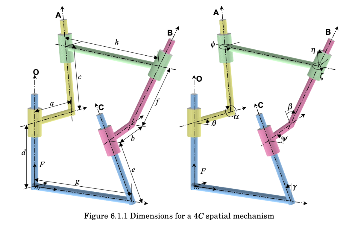
The Mechanism parameters are taken from:[1] CHANG, Da - Yu, et al . KINEMATIC AND STATIC ANALYSIS OF 4 C SPATIAL MECHANISMS . 1998. Tesis Doctoral . University of California, IrvineFigure 6.2.2See the link or the figure itself below:

In[]:=
(*linklengthparameters*)a=2;b=-3;g=-5;h=4;(*linkorientationparameters*)α=30*Degree;β=-225*Degree;γ=-240*Degree;η=55*Degree;
Position Equation
Position Equation
The position equation is obtained by describing the successive translations and rotations of a coordinate system following the mechanism geometry in a fixed position.The following figure was used to derive the loops O-A-B and O-C-B, which are mathematically reflected with the products of the transformation matrices, T1.T2.T3.T4 and T5.T6.T7.T8, respectively.The condition of loop closure, i. e. Pos1=Pos2, is imposed through the Objective Function 1.
In[]:=
Clear[θ,c,ϕ,e,ψ,f,ζ];T1=Tz6[θ];T2=Tz1[a].Tz4[α];T3=Tz3[c].Tz6[ϕ];T4=Tz1[h].Tz4[η];T5=Tz1[g].Tz4[γ];T6=Tz3[e].Tz6[ψ];T7=Tz1[b].Tz4[β];T8=Tz3[f].Tz6[ζ];Pos1=T1.T2.T3.T4;Pos2=T5.T6.T7.T8;OF1=;(*ObjectiveFunction1writtenasnon-linearleastsquares*)
4
∑
j=1
4
∑
i=1
2
(Pos1[[i,j]]-Pos2[[i,j]])
Position Equation Solution
Position Equation Solution
Initial Solution for the Position Equation
Initial Solution for the Position Equation
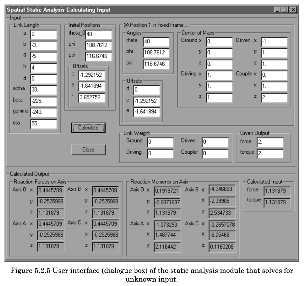
Theinitialvaluesoftheunknownsc,f,e,ϕ,ζandψweretakenfromtheInitialPositionssectionofthefollowingfiguretakenfromreference[1]:
Total Solution for the Solution Equation
Total Solution for the Solution Equation
The FindMinimum command is iteratively applied above to solve the condition of loop closure, Pos1=Pos2, by minimizing the objective function OF1 for each of the 360 degrees of a complete revolution.
For each iteration, the initial values are taken from the immediately previous iteration.
For each iteration, the initial values are taken from the immediately previous iteration.
Joint Offsets and Angles Plots
Joint Offsets and Angles Plots
The obtained plots above are equivalent to the plots given in reference [1]. This allows to conclude that the calculated output join offsets and angles are correct.
Velocity equation
Velocity equation
Velocity equation Solution
Velocity equation Solution
Initial Solution for the Velocity Equation
Initial Solution for the Velocity Equation
Total Solution for the Velocity Equation
Total Solution for the Velocity Equation
Velocity Plots
Velocity Plots
Animation
Animation