The problem of distributed consensus arises in networked systems where multiple autonomous agents or nodes must agree on a single data value or course of action despite polarized opinions, varying attitudes, possible communication delays, failures, or faulty participants. My project aims to analyze which conditions result in a certain type consensus, or in the least amount of time. I also explore how to optimize social networks in order to not only reach consensus, but also try and achieve desirable consensus.
Analyzing opinion dynamics across social networks, as well as how different factors could act as obstacles or delays to community reaching consensus really interested me. I wanted to explore this topic specifically in the context of peoples’ environmental concern, and simulate the different ways in which favourable consensus could be achieved, which ideally ends with everyone in the social network considered to ‘have environmental concern’ above a certain threshold.
Analyzing opinion dynamics across social networks, as well as how different factors could act as obstacles or delays to community reaching consensus really interested me. I wanted to explore this topic specifically in the context of peoples’ environmental concern, and simulate the different ways in which favourable consensus could be achieved, which ideally ends with everyone in the social network considered to ‘have environmental concern’ above a certain threshold.
Introduction
Introduction
In ‘The Problem of Distributed Consensus’ by Stephen Wolfram, he says “in any decentralized system with computers, people, databases, measuring devices or anything else one can end up with different values or results at different ‘nodes’. But for all sorts of reasons one often wants to agree on a single ‘consensus’ value, that one can for example use to ‘make a decision and go on to the next step’. One issue is to make the algorithm as efficient as possible.... Another is to make it as robust as possible, for example with respect to random noise—or malicious errors—introduced at or between nodes.... The amount of random noise can be thought of as something like a temperature. And at least in certain cases there can be a “phase transition” so that below a certain ‘temperature’ there can be zero effect on the consensus output—implying robustness to a certain level of noise.”
Achieving consensus is difficult because it requires the system to tolerate faults while guaranteeing that all non-faulty nodes reach the same decision without contradictions. Consensus could also be hindered by lack of connection or agreement between two different clusters of the network. This requires further analysis to understand and model why different types of social networks may or may not reach a certain type of consensus. Classical formulations, such as the Byzantine Generals Problem, highlight the complexity of reaching agreement when some participants may behave maliciously or unpredictably, thus requiring further investigation into what conditions, patterns and community structures within a social network affect the efficiency of consensus reached.
Achieving consensus is difficult because it requires the system to tolerate faults while guaranteeing that all non-faulty nodes reach the same decision without contradictions. Consensus could also be hindered by lack of connection or agreement between two different clusters of the network. This requires further analysis to understand and model why different types of social networks may or may not reach a certain type of consensus. Classical formulations, such as the Byzantine Generals Problem, highlight the complexity of reaching agreement when some participants may behave maliciously or unpredictably, thus requiring further investigation into what conditions, patterns and community structures within a social network affect the efficiency of consensus reached.
My Project’s Objective
My Project’s Objective
I wanted to achieve this by answering the following investigation questions:
1. How can a social network be represented as a graph most accurately?
2. How can peoples’ environmental attitudes and behaviours be condensed into two polarized opinions?
3. In what way can consensus be achieved computationally in a social network?
4. What happens if different parameters and variables are changed and how does this affect the end consensus reached as well as how efficient it was?
5. How can the unpredictability of human behaviour, error rates, or ‘stubbornness’ be factored into my computation?
6. How can I expand on my model to make it model a human social network as accurately as possible?
Creating the Initial Social Network Graph
Creating the Initial Social Network Graph
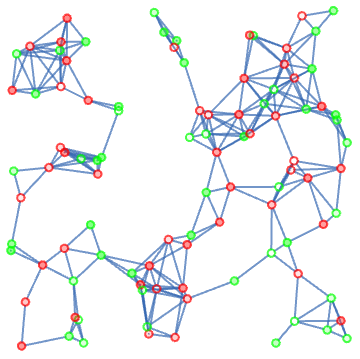
I started out by creating the first graph that will represent the social network. Each node represents a person in the social network, who forms connections through edges in the graph with other nodes. I used a nearest neighbour graph for my social network to realistically model how individuals are primarily influenced by their closest peers within a certain ‘radius’ of them, or those they happen to interact with in day-to-day life.
Generates a 2D graph by drawing edges from each node, represented by a randomly-generated co-ordinate, to those within a distance of 15 from them.
In[]:=
g = NearestNeighborGraph[RandomReal[100, {100, 2}], {All, 15}, VertexSize->2];v = VertexList[g];
Randomly generates, combines and then shuffles two subsets of random real numbers, one from 0-0.5 and the other from 0.5-1 inclusive.
In[]:=
env = RandomSample[Join[RandomReal[{0, 0.49}, Floor[Length[v]/2]], RandomReal[{0.5, 1}, Ceiling[Length[v]/2]]]];
Creates a condition such that nodes with environmental concern values <0.5 are assigned the colour red, and ≥0.5 are coloured green, with opacity adjustment and coloured edges.
In[]:=
valueToColourList[vals_] := Map[ If[# < 0.5, Directive[Red, Opacity[#], EdgeForm[Red]], Directive[Green, Opacity[# - 0.5], EdgeForm[Green]] ] &, vals];
Creates a function to generate the coloured social network graph based on env values of the randomly-generated nearest neighbour graph.
In[]:=
generateGraph[vals_, vertices_] := NearestNeighborGraph[ vertices, {All, 15}, VertexStyle -> Thread[vertices -> valueToColourList[vals]], VertexSize -> 2, VertexLabels -> None, ImageSize->Small];
Displays the final social network graph.
generateGraph[env,v];
Out[]=
Simulating the Achievement of Consensus
Simulating the Achievement of Consensus
As seen in actual social networks, people’s opinions and attitudes tend to be influenced by those of their surrounding acquaintances or connections.This could happen due to social conformity, normative influence, and the desire for social acceptance, where individuals adjust their opinions to align with perceived group norms.I tried to emulate this by creating a function that would mathematically compute a new environmental concern value for each node based on the environmental concern values of its direct connections, all in the same time-step. To do so, I used the formula of Distributed Average Consensus with Least-Mean-Square Deviation to accurately simulate such behaviour at each function call:xᵢ(t + 1) = xᵢ(t) + ∑ⱼ∈𝒩ᵢ Wᵢⱼ ( xⱼ(t) – xᵢ(t) )This formula adjusts the EnvironmentalConcern value of each node in the next time step, based on its value in the current time step and the values of all of its directly connected neighbours, with equal weight given to each of them. If a node is currently green, and if most of the surrounding nodes are significantly red, its EnvironmentalConcern value will be reduced overall. If it is reduced far enough and dips below the threshold, its colour will change from green to red. The same goes for an increase in the value of a red node which turns it green, and the opacities are accordingly adjusted.
Implements above formula for each node in a graph to adjust its env value based on those of all its directly connected neighbours.
In[]:=
updateValues[graph_, values_, vertices_] := Module[{newValues, neighbors, wij, xi, index}, newValues = Table[ neighbors = AdjacencyList[graph, vertices[[i]]]; xi = values[[i]]; If[Length[neighbors] == 0, xi, wij = 1/Length[neighbors]; xi + Sum[( index = FirstPosition[vertices, neighbors[[j]], Missing[]]; If[MissingQ[index], 0, wij * (values[[index[[1]]]] - xi) ]), {j, Length[neighbors]} ]], {i, Length[vertices]}]; newValues];
Creates a condition to check whether consensus has been reached in the social network ie. all nodes are either green or red.
In[]:=
consensusQ[vals_] := AllTrue[vals, # < 0.5 &] || AllTrue[vals, # >= 0.5 &];
Allows the repeated calls of the updateValues function for a particular graph and returns the updated graph and env values at each time-step.
In[]:=
createSim[state_, vertices_] := With[{newVals = updateValues[state[[1]], state[[2]], vertices]}, {generateGraph[newVals, vertices], newVals}];
Calls createSim for social network graph created until consensus is reached, or if not, until a maximum of 2000 time-steps.
In[]:=
graphs=NestWhileList[createSim[#,v]&,{generateGraph[env,v],env},Not[consensusQ[#[[2]]]]&,1,2000];
Extracts graphs at each time-step and finds how many repetitions were required to reach consensus.
In[]:=
graphSequence=graphs[[All,1]];Length[graphSequence]
Out[]=
426
Displays an animation of an updated graph at each time-step for easy visualization of how consensus is reached.
Out[]=
This simulation is representative of a social network with 100 people influenced equally by all their direct neighbours. We see that it is reaching a red consensus. This is not quite a favourable outcome, considering that in real-world society, an idealistic outcome would be that everyone achieves positive environmental attitudes/has environmental concern. I will later explore ways to try and maximise chances of achieving this preferable outcome in the following sections.
Reducing Nodes/Number of People in the Social Network
Reducing Nodes/Number of People in the Social Network
What happens if we look at a smaller community, instead of 100 people? Does reducing the number of people significantly decrease/increase the time required to reach consensus? Does it change the type of consensus finally achieved?
Created the same nearest neighbour graph but with only 50 nodes (25 green and 25 red):
Runs simulation on smaller graph.
This smaller community reached consensus more efficiently in only 34 time-steps, compared to 426 for the 100 people network! However, this difference could also be because of the fact that the nodes are more closely connected/closely-knit and a neighbour is still considered to be within 15 units within you.
To make it a fairer test I reduced the distance requirement for a neighbour/direct connection to be formed between nodes to 11, since the number of people has been halved. I did this in order to more closely emulated what happens if you look at a smaller sub-section of a community, since in a smaller network one would not form connections within the same radius of themselves. I chose 11 as it was the minimum distance while testing for the graph to be fully connected/not have small fragments.
To make it a fairer test I reduced the distance requirement for a neighbour/direct connection to be formed between nodes to 11, since the number of people has been halved. I did this in order to more closely emulated what happens if you look at a smaller sub-section of a community, since in a smaller network one would not form connections within the same radius of themselves. I chose 11 as it was the minimum distance while testing for the graph to be fully connected/not have small fragments.
Creates smaller social network graph that allows nodes to form connections with neighbours within a distance of 11 from them.
Redefines simulation functions according to new distance requirement and runs simulation on new graph.
Compared to the first smaller graph which took 34, this new graph which more accurately models a smaller community only took 11 time-steps to achieve consensus.
However, we see that with the more realistic distance requirement, the social network reaches red consensus, whereas the first time around the smaller graph had reached green consensus.
This tells us that efficiency/speed might sometimes compromise on the desirability of the result, which closely replicates actual societies as smaller, more tightly connected communities would propagate an opinion quickly, but it may not necessarily be what is more widely accepted by the entire social network.
To better understand what may be causing the differences in these outcomes, I decided to analyse more closely the distributions of the number of connections for each node across all three graphs above: the 100 people network, the 50 people idealistic network, and the 50 people more realistic network. This was so that I could draw conclusions on the edge distributions in each graph and see how similar or different they were.
First we analyse the number of connections for each vertex in the smaller graph with the distance condition 15:
However, we see that with the more realistic distance requirement, the social network reaches red consensus, whereas the first time around the smaller graph had reached green consensus.
This tells us that efficiency/speed might sometimes compromise on the desirability of the result, which closely replicates actual societies as smaller, more tightly connected communities would propagate an opinion quickly, but it may not necessarily be what is more widely accepted by the entire social network.
To better understand what may be causing the differences in these outcomes, I decided to analyse more closely the distributions of the number of connections for each node across all three graphs above: the 100 people network, the 50 people idealistic network, and the 50 people more realistic network. This was so that I could draw conclusions on the edge distributions in each graph and see how similar or different they were.
First we analyse the number of connections for each vertex in the smaller graph with the distance condition 15:
Plots a line graph with vertices on the x-axis and the number of node connections on the y-axis.
Next we analyse the number of connections for each vertex in the smaller, realistic graph with the distance condition 11:
Plots a line graph with vertices on the x-axis and the number of node connections on the y-axis.
We see that the edge distribution of the small graph with distance condition 11 has a smaller range of values/deviates less from the average than the small one with distance condition 15. This may be because the range of values possible for the latter are more spread out and unpredictable, and thus it is not as accurate for representing a smaller, closely-connected community. Barring this, the overall distribution patterns are quite similar. This shows that the lesser spread of the connection values in the reduced distance condition graph cause it to achieve consensus more quickly and efficiently since other factors like edge distribution patterns across graphs are quite similar.
Next we analyse the number of connections for each vertex in the big graph with 100 nodes:
Plots a line graph with vertices on the x-axis and the number of node connections on the y-axis.
The overall edge distribution patters on the bigger graph have similar repetitions to those of the smaller ones with large fluctuations. Overall, , we can say that for a smaller number of people, the conclusion remains that if forming a more closely-knit community, the reduction in the number of time-steps is exponentially reduced due to lesser room for conflicting opinions.
But is there a way we can quantify how ‘closely-knit’ a community actually is in order to strengthen our conclusion that the first smaller graph, with the same distance requirement is more closely-knit then the bigger community and is thus quicker to reach consensus in most cases?
The overall edge distribution patters on the bigger graph have similar repetitions to those of the smaller ones with large fluctuations. Overall, , we can say that for a smaller number of people, the conclusion remains that if forming a more closely-knit community, the reduction in the number of time-steps is exponentially reduced due to lesser room for conflicting opinions.
But is there a way we can quantify how ‘closely-knit’ a community actually is in order to strengthen our conclusion that the first smaller graph, with the same distance requirement is more closely-knit then the bigger community and is thus quicker to reach consensus in most cases?
Finds clusters/communities within first small graph, finds the average number of connections within each of the communities and also how many communities there are.
Does the same for the reduced distance condition smaller graph.
Does the same for the bigger 100 people graph.
We clearly see, through these results, that the both the smaller, 50 people networks are the most connected and closely-knit as:
1) They has fewer sub-communities than the bigger network (4 and 5 vs. 8) showing they are more closely-structured.
2) Each node in the communities has a much higher average number of connections showing it is more closely-connected. (7.85 and 4.9 vs 4.67)
This investigation thus strengthens or backs my hypothesis that smaller networks will tend to reach consensus quicker since they are more inter-connected and closely-knit.
1) They has fewer sub-communities than the bigger network (4 and 5 vs. 8) showing they are more closely-structured.
2) Each node in the communities has a much higher average number of connections showing it is more closely-connected. (7.85 and 4.9 vs 4.67)
This investigation thus strengthens or backs my hypothesis that smaller networks will tend to reach consensus quicker since they are more inter-connected and closely-knit.
Plotting Green and Red Nodes Over Time in Simulation
Plotting Green and Red Nodes Over Time in Simulation
Each community and social network obviously differs in structure and distribution, thus causing differences in the number of time-steps required to reach consensus. I decided to create 5 different interconnected graphs representing fully connected communities and run the simulations on each of them in order to try and get as much of an average conclusion with as large a scope for evaluation as possible.
Creates 5 randomly generated nearest neighbour social network graphs. Below is the code for the first graph which I repeated for 5 different social network graphs.
Runs consensus simulation on all 5 graphs.
Compiles all the generated graphs at each time-step into one list.
Counts all the red and all the green nodes for each simulation of each graph.
Creates a helper function to pad the lists and compute the average counts of all 5 graphs.
I now wanted to make a line graph for both the red nodes, and the green nodes. This would display the number of green nodes and red nodes over each time-step for all 5 graphs, and then also compute the average of the 5 graphs as a blue line and display it. This would be in order to represent the dynamics more holistically due to sampling across different initial conditions, since there are a lot of variations between each social network’s consensus no matter how similarly they may be structured.
Computes the range of x-values and y-values I want to display on my graph’s axes.
Plot 5 red lines for all 5 graphs and blue line graph for average.
Does the same for the green nodes over time.
From these graphs we observe that the green nodes over time in one graph, represents a line exactly opposite to the one on the red graph. This may be because green is the red line reflected on the line y=convergence point. In this case the convergence point for all the graphs is 50 since they begin with a half-and-half split.
We can also see some of the graph flatten out before others, showing they needed fewer time-steps to approach consensus. The large difference in the number of time-steps causes an overall generally horizontal average line with slight fluctuations for both coloured nodes.
It’s really interesting that none of the lines are moving in a fixed direction. There are changes between upward and downward movement for each of the nodes and certain intervals, and very small fluctuations towards the beginning, until we later on see a big increase or decrease in the counts before they flatten out to become 0 or 100. In society, we also see that two polarized opinions would initially create a sense of uncertainty or indecision between the clear majority for a while, until eventually one opinions gain just enough momentum to then rapidly convert the rest of the community.
One line however, representing graph 3, is noticeably different from the rest. We see that neither the red or the green nodes become or 100, and their counts stop changing once they reach 50. This made me curious as to why this graph failed to reach consensus, since it was a fully connected graph with no fragments or isolated nodes, and I decided to run the consensus function on it to visualize the simulation and what was causing the failure.
We can also see some of the graph flatten out before others, showing they needed fewer time-steps to approach consensus. The large difference in the number of time-steps causes an overall generally horizontal average line with slight fluctuations for both coloured nodes.
It’s really interesting that none of the lines are moving in a fixed direction. There are changes between upward and downward movement for each of the nodes and certain intervals, and very small fluctuations towards the beginning, until we later on see a big increase or decrease in the counts before they flatten out to become 0 or 100. In society, we also see that two polarized opinions would initially create a sense of uncertainty or indecision between the clear majority for a while, until eventually one opinions gain just enough momentum to then rapidly convert the rest of the community.
One line however, representing graph 3, is noticeably different from the rest. We see that neither the red or the green nodes become or 100, and their counts stop changing once they reach 50. This made me curious as to why this graph failed to reach consensus, since it was a fully connected graph with no fragments or isolated nodes, and I decided to run the consensus function on it to visualize the simulation and what was causing the failure.
Checks that the graph never reaches consensus.
Find the time-step at which the nodes stop changing colour, known as the stabilisation time-step.
Visualizes the last couple of time-steps until stabilization.
Upon visualizing the last two time-steps until stabilization, we see that the polarized communities stop changing colour beyond a certain node that is acting as a bridge between two clusters.
We can see that the cluster that is failing to change colour to green and propagating the consensus further is very closely interconnected and tightly packed, and the high opacity values of all the nodes within it also show that it would be difficult to adjust significantly. The combination of these factors probably halted the consensus and didn’t allow the green to spread further.
In society too, very strongly-connected and opinionated clusters may show such ‘stubbornness’ thereby preventing the entire community from achieving consensus.
We can see that the cluster that is failing to change colour to green and propagating the consensus further is very closely interconnected and tightly packed, and the high opacity values of all the nodes within it also show that it would be difficult to adjust significantly. The combination of these factors probably halted the consensus and didn’t allow the green to spread further.
In society too, very strongly-connected and opinionated clusters may show such ‘stubbornness’ thereby preventing the entire community from achieving consensus.
Fragmented and Isolated Graphs/Communities
Fragmented and Isolated Graphs/Communities
Until now, all of my investigations were being conducted on fully connected communities, which are usually almost guaranteed to reach consensus. But what happens if there are isolated sections within a community? Do they often not reach consensus? Which types of fragmented communities fail to reach consensus? What changes or additions could push such graphs towards overcoming dis-consensus?
Two Fragments
Two Fragments
I began by creating a graph with two fragments, representing two disconnected factions in a community/social network.
Randomly generates a nearest neighbour social network graph.
If consensus is never reached, there must be a maximum number of time-steps the simulation should be run for to prevent an infinite loop. In this case, I picked 200.
Runs updateValues consensus simulation on the two-fragmented graph up to 200 times.
Visualizes the progression of each fragment until the maximum number of time-steps.
Through the animation, we see that after a certain point the nodes do not change in colour. One faction has reached green consensus, and one red, but the lack of connection between them causes overall dis-consensus.
I decided to graph the the number of green and red nodes in this simulation over time until a little bit after the point when the nodes eventually stop changing colour, or the stabilization time-step.
I decided to graph the the number of green and red nodes in this simulation over time until a little bit after the point when the nodes eventually stop changing colour, or the stabilization time-step.
Counts green and red nodes within the graph at each time-step.
Creates a condition to detect the time-step at which consensus was reached.
In this case, the graph never reaches consensus.
Makes a function to find the true stabilisation point, or the point at which the colours (environmental concern values here) stop changing.
This graph takes 43 time-steps to reach consensus within each fragment, probably because each fragment is smaller than a fully connected graph with 100 nodes so they can stabilize within themselves quicker.
Calculates padded end step to be 120% of stabilisation step to show horizontal line depicting no more change on the graph.
Defines final end step for plotting.
Trims all count and time-step values to end step.
Defines final value for horizontal line extension.
Outputs a formatted and styled, combined plot for count of both red and green nodes on y-axis vs time-step on the x-axis.
From this graph, we see that the overall difference in the entire social network for the green and red node count until stabilization is quite negligible. This because one approximate half or fragment became green and one red, balancing out the counts in the end with slight fluctuations. The end majority is primarily decided within the initial upwards or downwards spikes in the first couple of time-steps. This observation is the opposite to our observations in the wholly connected graph, where the final majority was decided towards the end and not the beginning.
Three Fragments
Three Fragments
Randomly generates a nearest neighbour social network graph (with 3 fragments).
Runs the same code above for the new three-fragmented graph and runs the consensus simulation.
Visualizes the progression of each fragment until the maximum number of time-steps.
Counts green and red nodes within the graph at each time-step.
Creates a condition to detect the time-step at which consensus was reached.
Finds the true stabilisation point, or the point at which the colours (environmental concern values here) stop changing.
In this one, we see compared to the graph with two larger sub-communities, this one reaches consensus or stabilization within its sub-groups within only 15 time-steps compared to 43. We can only assume this is because two of the factions are much smaller, allowing them to stabilise quicker within themselves as seen in our previous investigation where we reduced the number of people/nodes.
Calculates padded end step to be 120% of stabilisation step to show horizontal line depicting no more change on the graph.
Defines final end step for plotting.
Trims all count and time-step values to end step.
Defines final value for horizontal line extension.
Displays final combined, styled plot.
From this graph, we see that the green nodes slightly decrease and then increase over time, while the opposite happens for the red nodes.
Isolated Nodes Within a Graph
Isolated Nodes Within a Graph
The last type of graph I investigated within these fragmented communities was one which included absolute isolation. This meant including people with only 1-2 connection(s), or even 0. I thought it would be interesting to investigate such a situation and what would happen in such a simulation. Would those vertices be the only one preventing consensus or would there be other factors as well?
Randomly generates a nearest neighbour social network graph (with smaller fragments and completely isolated nodes).
Runs the same code above for the isolated graph and runs the consensus simulation.
Visualizes the progression of each fragment until the maximum number of time-steps.
Counts green and red nodes within the graph at each time-step.
Creates a condition to detect the time-step at which consensus was reached.
Finds the true stabilisation point, or the point at which the colours (environmental concern values here) stop changing.
In this one, we see compared to the first 2 fragmented graphs, this isolated graph reaches consensus or stabilization within its sub-groups within a much larger number of time-steps, 166. When looking at the visualization of the simulation, we see that this delay is caused due to the fact there are two clusters within the largest connected community, and it takes very long for the green consensus to transfer across this connection to the red cluster, and even after it does so with the first node, the transfer ends there and consensus is not achieved in the rest of the large cluster.
This could represent delay in uptake or unwillingness to change if your closer sub-community is of an opposite opinion, which is we see only the node directly connected to the other cluster change to green and not the rest after that.
This could represent delay in uptake or unwillingness to change if your closer sub-community is of an opposite opinion, which is we see only the node directly connected to the other cluster change to green and not the rest after that.
Calculates padded end step to be 120% of stabilisation step to show horizontal line depicting no more change on the graph.
Defines final end step for plotting.
Trims all count and time-step values to end step.
Defines final value for horizontal line extension.
Displays final plot.
For this graph, we see a very interesting progression of counts over time. Starting at 50 nodes distributed per color, we once again see that the green and red nodes are mirrored on the line y=50. We see a pattern of increasing and then decreasing at different intervals, creating an almost geometric progression until the counts stabilize. The intersection as the lines cross each other show that the fluctuations are repetitive as each small fragment and cluster in the larger community changes colour, until they eventually stop and level out.
Consensus Threshold
Consensus Threshold
Upon reaching consensus, I wanted to analyse the final environmental concern values and how similar or different they were, both in a graph that reaches red consensus and green consensus. I first got a list of all of the final opacity values in the consensus graphs. The below is for a red consensus graph:
Extracts the final opacity values in the last time-step once consensus is reached.
We see that all of the opacity values are within the range of around 0.48-0.49, barely crossing the threshold of 0.5. Even a small change could cause them all to turn green.
Below is the same for a green consensus graph:
Below is the same for a green consensus graph:
Once again, the values range from 0.5-0.55, very close to the threshold! However, we see that overall in the green consensus graph, that the final values are a little further from the threshold than in the red consensus graph and would be harder to nudge back below the threshold. This is also representative of a real social network, because once you achieve environmental concern and become passionate about it, there is a smaller chance you would go back to not having it.
However, this investigation raises the question- is consensus in this case actually consensus? Consensus here is considered achieved the moment everyone is the same colour, not considering the fact that it simply uses the minimum effort/energy route and might not affect people opinions or attitudes that much since the values in a red consensus graph are barely different from a green consensus graph.
This leads me to ask: would continuing to run the simulation even after ‘coloured consensus has been achieved’ further affect the values, or further increase and decrease them? This might be useful in the case of green consensus for EnvironmentalConcern, by improving people’s environmental attitudes even further than the required threshold, rather than simply fulfilling the requirement of ‘consensus’. I investigated this on the same green consensus graph above, running the simulation until the actual environmental concern values all became the same, and not just the colour:
However, this investigation raises the question- is consensus in this case actually consensus? Consensus here is considered achieved the moment everyone is the same colour, not considering the fact that it simply uses the minimum effort/energy route and might not affect people opinions or attitudes that much since the values in a red consensus graph are barely different from a green consensus graph.
This leads me to ask: would continuing to run the simulation even after ‘coloured consensus has been achieved’ further affect the values, or further increase and decrease them? This might be useful in the case of green consensus for EnvironmentalConcern, by improving people’s environmental attitudes even further than the required threshold, rather than simply fulfilling the requirement of ‘consensus’. I investigated this on the same green consensus graph above, running the simulation until the actual environmental concern values all became the same, and not just the colour:
Creates a condition for consensus that checks that all env values have become the same.
Runs the simulation until this new consensus condition is reached or until a maximum of 100,000 time-steps.
Extracts final env values after running new simulation.
Theoretically, the value reached by doing this would be the highest possible, optimized uniform favourable consensus value a social network would be able to reach. Thus, the value 0.514913 was reached by evening out the higher-value nodes with the lower-value nodes until they all became equal and there was no further room to adjust.
While further optimization may not be possible, we see that a green consensus can be considered better than the initial graph with both red and green values, ending in a beneficial or preferable result.
However, there are of course downsides to The Problem of Distributed Consensus, as there is always a risk of the unwanted opinion/red consensus being achieved. I wanted to find a way to try and minimize or remove the chance of getting such a result and optimize the consensus reached.
While further optimization may not be possible, we see that a green consensus can be considered better than the initial graph with both red and green values, ending in a beneficial or preferable result.
However, there are of course downsides to The Problem of Distributed Consensus, as there is always a risk of the unwanted opinion/red consensus being achieved. I wanted to find a way to try and minimize or remove the chance of getting such a result and optimize the consensus reached.
Starting Without an Even Split, Connection Dsitributions, Node Weightage and Skewing
Starting Without an Even Split, Connection Dsitributions, Node Weightage and Skewing
Creating the Majority Graph and Simulating Consensus on it
Creating the Majority Graph and Simulating Consensus on it
My investigations till now began with these simulations starting with an equal number of green and red nodes. But what happens if you start with a slight majority in one colour?
I decided to investigate this with a 51% vs 49% split between colours as it would be the most efficient to run and easiest to investigate. I began my investigation with a social network with a majority of the unfavourable opinion, with 51% red and green 49%.
I decided to investigate this with a 51% vs 49% split between colours as it would be the most efficient to run and easiest to investigate. I began my investigation with a social network with a majority of the unfavourable opinion, with 51% red and green 49%.
Randomly generates a nearest neighbour social network graph.
Generate 49 red (<0.5) and 51 green (⩾0.5) values instead of a 50/50 even split and then generates the coloured graph implementing those env values.
Runs the consensus simulation on the majority graph.
We see the number of time-steps required to reach consensus is 164, much smaller than what a 50/50 graph would take since there is already a slight bias, making it quicker and easier to pick a side to reach consensus for. In this case, the majority colour is red, resulting in unfavourable consensus.
Is there a way to somehow shift the consensus to a more favourable outcome, in this case green, even with the unfavourable majority? There were three ways in which I investigated this:
Is there a way to somehow shift the consensus to a more favourable outcome, in this case green, even with the unfavourable majority? There were three ways in which I investigated this:
Manipulating the Number of Connections in Favour of Green Consensus
Manipulating the Number of Connections in Favour of Green Consensus
The first was by assigning all of the nodes with highest number of connections/highest VertexDegree to the minority colour, in this case green. These would represent more influential people in society, who of course have more impact on consensus decisions:
Randomly generates a nearest neighbour social network graph and finds the length of its vertex list.
Finds the number of connections for each node and transposes its corresponding VertexDegree value to each node:
Sorts the VertexDegree data in descending order, so the nodes with the highest connections were first and then assigns the first 49 vertices the green colour and the next 51 (lowest connections) the red colour.
Re-generates 49 red and 51 green values and assigned them a random range of values based on defined thresholds:
Displays graph.
One general observation, we can make on this graph is that similar colours tend to be grouped together or next to each other in clusters more so than in the randomly-generated graphs due to the sorting by VertexDegree.
This can also be seen in society as more influential people (green) tend to interact with each other and form ‘cliques’.
This can also be seen in society as more influential people (green) tend to interact with each other and form ‘cliques’.
Runs consensus simulation on the majority graph with manipulated VertexDegrees.
On running the simulation on this graph, we see positive results, as the consensus reached is not only green, but also more efficient than a regular simulation with a 50/50 graph as it is reached in fewer time-steps of only 75. This solution was successful, since green nodes get to adjust a greater number of node’s values upwards due to the higher number of connections while red nodes can only bring down the values of a few!
Skewing the Environmental Concern Values Upwards
Skewing the Environmental Concern Values Upwards
For the third solution, I am starting once again with 51 red nodes and 49 green nodes, I generated the initial graph such that the EnvironmentalConcern values for both the red and green nodes were predefined in a way that were skewed higher/upwards.
Randomly generates a nearest neighbour social network graph with 51% majority red nodes and 49% green.
Assigns all red nodes relatively high values 0.25-0.5 and all the green nodes, in minority, a high value of 0.75-1, slightly skewed towards the higher end of the range and displays the graph.
Runs consensus simulation on the slightly skewed graph.
Once again, this solution too is successful as it is another way to bias or intensify opinions towards a green consensus from the very outset, allowing the social network to overcome the red majority and achieve favourable consensus. Moreover, it does so extremely efficiently in only 22 time-steps.
I now wanted to explore if further intensifying the skew upwards could be a potential solution to the problem I faced earlier with the fragmented graphs, wherein the two factions reached two different consensus. I thought so since this had been the most efficient solution by far, and it could also pre-emptively determine or guarantee favourable results.
I now wanted to explore if further intensifying the skew upwards could be a potential solution to the problem I faced earlier with the fragmented graphs, wherein the two factions reached two different consensus. I thought so since this had been the most efficient solution by far, and it could also pre-emptively determine or guarantee favourable results.
Randomly generates a nearest neighbour social network graph with 51% majority red nodes and 49% green.
Now, I skewed the values even higher upwards from 0.4-0.5 for red and 0.9-1 for green in order to create enough of an incentive for both fragments to try and reach green consensus.
Assigns all red nodes very high values 0.4-0.5 and all the green nodes, in minority, a high value of 0.9-1, highly skewed towards the higher end of the range and displays the graph.
Runs consensus simulation on the highly-skewed, fragmented graph.
This solution clearly worked, since not only do both factions end up reaching green consensus, but the solution is achieved within only 12 time-steps!
In my opinion, combining each of the three methods would optimize the results as much as possible, with the last solution of skewing being the most efficient. This would prove that a combination of social influence, as well as conditions in society showing a higher inclination towards environmental consciousness play a big role.
In my opinion, combining each of the three methods would optimize the results as much as possible, with the last solution of skewing being the most efficient. This would prove that a combination of social influence, as well as conditions in society showing a higher inclination towards environmental consciousness play a big role.
Adding Error Rates
Sometimes, as observed in most human social networks, some nodes or ‘people’ may not succumb to peer pressure. This is referred to as an error rate, where no matter what your connections’/neighbours’ opinions maybe, in each timestep some people’s opinions or environmental concern values do not change.
In order to investigate this, I took 5 fully connected social networks, and ran a simulation with a built-in, customisable error rate on them. I used RandomSample[] to get the specified percentage of vertices randomly picked to be the ‘error nodes’ which do not adjust their environmental concern values based on their neighbours:
In order to investigate this, I took 5 fully connected social networks, and ran a simulation with a built-in, customisable error rate on them. I used RandomSample[] to get the specified percentage of vertices randomly picked to be the ‘error nodes’ which do not adjust their environmental concern values based on their neighbours:
Runs the updateValues function on all nodes in each time-step except a randomly sampled percentage of the nodes, or ‘error nodes’, which do not adjust their env values in each time-step.
Runs the consensus function with a 5% error rate and displays results.
We see that the efficiency of consensus is significantly reduced, as this same graph took only 426 time-steps to run with an error rate (at the beginning of the essay) compared to 629 with the 5% error rate. However, the error rate was not large or significant enough to change the colour of consensus reached, which is still red.
In human social networks too, ‘stubbornness’ displayed by certain people or their unwillingness to change their opinions based on those around them is observed, which is what I aimed to represent with this error rate. I wanted to see the different outcomes of as many error rates as possible in terms of the number of time-steps required for consensus as well as the colour of consensus reached. I decided to visualize this pattern this using a line graph.
In human social networks too, ‘stubbornness’ displayed by certain people or their unwillingness to change their opinions based on those around them is observed, which is what I aimed to represent with this error rate. I wanted to see the different outcomes of as many error rates as possible in terms of the number of time-steps required for consensus as well as the colour of consensus reached. I decided to visualize this pattern this using a line graph.
Creates a function to run the consensus function on a specified graph and its list of env values and nodes.
Runs each computation separately since it is a heavy simulation for 5 different graphs.
Extracts required data on the required time-steps for consensus.
Extracts required data on the colour of consensus reached .
Computes the average time-step values from all the 5 graphs to give a more accurate and overarching representation.
Finds the most common majority consensus colours from all 5 graphs for a particular error rate to display on the average line of the graph.
Converts majorityColours into directives to display them as graphics as PlotMarkers on the average line graph:
I then had to create a plot of the green and red nodes separately, since one line in a ListLinePlot cannot have more than one type/colour of marker.
Defines the error rates to run the simulation with from 5 to 95 at intervals of 5.
Generates the data for the plot markers on the graph based on the majority consensus colour reached between all 5 graphs at each error rate.
Plots only the green disks for the plot markers representing the graphs which reached green consensus:
Plots only the red disks for the plot markers representing the graphs which reached red consensus:
Defines points for the error rates x-axis of the line graph and transpose the data to fit this distribution:
Defines x and y-axis limits based on maximum time-steps taken:
Plots the line graph for the 5 graphs’ simulations and then the average line separately since I had different style specifications and plot markers present.
Upon analysing the graph, we see that most often, we get a favourable outcome or green consensus for most error rates, most especially at the higher error rates.
Regarding time-steps required, there are constant spikes representing that in certain cases, higher percentage error rates may not necessarily result in greater time-steps. At around 65% we see a very sharp decline, and at 75%, we see a steep increase in time required to consensus, which flattens out a bit at 85%.
Regarding time-steps required, there are constant spikes representing that in certain cases, higher percentage error rates may not necessarily result in greater time-steps. At around 65% we see a very sharp decline, and at 75%, we see a steep increase in time required to consensus, which flattens out a bit at 85%.
Extension: Modelling Human Networks More Accurately with Social and Economic Parameters
Extension: Modelling Human Networks More Accurately with Social and Economic Parameters
Creating the Graphs, Variables and Thresholds
Creating the Graphs, Variables and Thresholds
I wanted to further my investigation by trying to more closely and accurately model actual people in real social networks.
Randomly generates nearest neighbour social network graph.
When thinking about what the most important aspects or attributes of people I wanted to include to represent each person when it came to their environmental attitudes, I was able to narrow it down to 3: environmental concern, the most crucial representing personal passion/drive, cost densitivity representing economic incentive since one of the main drawbacks to adopting environmental alternatives is the higher costs, and peer pressure, since most decisions in a community or social network are influences by triggers for compliance due to social desirability.
Assigns a random value from 0 to 1 to two out these three variables:
I then had to create another value cost factor, which reversed the effect of cost sensitivity. This is because, the higher one’s costSensitivity, the less environmentally motivated they are. Thus, for my calculations, it would be more efficient and accurate to use costFactor since cost sensitivity is negatively correlated to a person’s overall green motivation:
Calculates costFactor based on person’s costSensitivity.
I spent a lot of time thinking about the most accurate and efficient way to represent peer pressure in the context of this simulation. The following code is for my initial calculation of peer pressure and then also to call the function in each time-step during the simulation.
I found one of the most important factors when assessing PeerPressure is that it varies from person to person. You would give more weightage or importance to something your best friend or parents, or someone you closely interact with everyday over an acquaintance or colleague. This is simply because of the fact that you see or talk to them more often, making their opinions and beliefs subconsciously affect you more.
Therefore, I began by assigning each neighbour/connection a default weightage of one. I then chose one node to be considered your ‘strongest tie’ with the highest weightage and the ‘weakest tie’ who could be someone you may not like the lowest weightage, and then another node with the ‘second strongest tie’ with a slightly lower weightage. The strongest tie has a weightage of 2.5-3, the second-highest 1.5-2 and the lowest 0.5-0.9.
I then decided to calculate the peer pressure value based on all the neighbour’s environmental concern values, by taking the weighted mean. This was because the environmental concern variable plays the most important role in how you are socially influenced into making sustainable choices:
I found one of the most important factors when assessing PeerPressure is that it varies from person to person. You would give more weightage or importance to something your best friend or parents, or someone you closely interact with everyday over an acquaintance or colleague. This is simply because of the fact that you see or talk to them more often, making their opinions and beliefs subconsciously affect you more.
Therefore, I began by assigning each neighbour/connection a default weightage of one. I then chose one node to be considered your ‘strongest tie’ with the highest weightage and the ‘weakest tie’ who could be someone you may not like the lowest weightage, and then another node with the ‘second strongest tie’ with a slightly lower weightage. The strongest tie has a weightage of 2.5-3, the second-highest 1.5-2 and the lowest 0.5-0.9.
I then decided to calculate the peer pressure value based on all the neighbour’s environmental concern values, by taking the weighted mean. This was because the environmental concern variable plays the most important role in how you are socially influenced into making sustainable choices:
Calculates peer pressure value for a person by taking weighted average of its neighbours envConcern values
When thinking about how important these factors were in comparison to each other, I began doing research on whether I should give them all equal weightage. I derived the weightages based on Ajzen’s (1991) Theory of Planned Behavior, giving the highest weight to environmental concern as attitudes strongly influence intent. I assigned a moderate weight to peer pressure informed by Goldstein et al. (2008), which showed that social norms significantly drive eco-actions and are powerful nudges, and a lower weight to cost sensitivity reflecting Thøgersen’s (2014) findings that while cost is a barrier, it does not motivate behavior positively.
Assigns weightages for the three variables in greenMotivation calculation.
I then used the following formula to calculate an overall variable green motivation to represent each person, which took into account in a weighted manner each of the three variables discussed above, where w1 + w2 + w3 = 1 (weights normalized):
Calculates peer pressure and green motivation for nodes based on the functions and formula above.
I then assigned a threshold for the different colours of each node, with green nodes having green motivation>=0.6, orange being >=0.4 and red being <0.4. The reason I chose this staggered list and these values, to represent low, medium, and high green motivation levels, is that it aligns with behavioural research that categorises attitudes or readiness into clear tiers for intervention. For example, <0.4 (red) indicates low motivation needing strong policy change, 0.4–0.6 (orange) reflects moderate motivation where nudge interventions are effective and can be implemented, and >0.6 (green) shows high motivation likely to result in eco-actions without intervention, similar to Likert scale interpretations and social threshold models.
I also then assigned the relative opacity values to each node based on the values and thresholds.
I also then assigned the relative opacity values to each node based on the values and thresholds.
Creates thresholds for assigning colours and opacities to nodes on the graph.
Plots the graph:
Creates an association for all the 4 values associated with each node, to access any value needed for computations easily:
Tests accessing all the attributes of the first node: {envConcern, costFactor, peerPressure, greenMotivation}
Tests getting all greenMotivation values from association for each node:
Conclusion
Conclusion
Through my project, I was able to reach a lot of conclusions about how social networks function and how they can reach consensus. Smaller communities are quicker to reach consensus, as are biased ones. The consensus outcome can be manipulated in favour of desirable outcomes by adding influential nodes which are more connected or weighted. A skewed social network also favours a certain consensus outcome. However, with no changes in these parameters, consensus achieved is the most stable, minimum energy solution required and doesn’t necessarily create a strongly opinionated final value as there isn’t much deviation from the threshold. This means that there is not necessarily a very strong change in the network’s environmental concern as the higher, ‘passionate’ people’s values are evened out closer to consensus.
To factor in more realistic aspects of human social networks, error rates add ‘stubbornness’ factors to the nodes and increase or sometimes decrease the time required for consensus to be achieved. The varying outcomes due to the random model accurately represent the fact that human decisions and biases are unpredictable by nature and cannot be represented by a single linear relationship.
To make the model more accurate in modelling real human networks, I added an extension implementing more parameters and variables. When applied to environmental concern in social networks, economic and social factors like cost sensitivity and peer pressure they are important factors that should be implemented in the simulation for consensus.
As further future exploration, error rates can also be modelled based on real-life applications of these variables. These variables, along with graph probability distributions can be changed to emulate different environments, such as rural and urban areas and then the differences can be analysed when running the simulation in each of the different areas.
Different shock factors such as activists, which have high environmental concern values and high weightages, fiscal policies on sustainability, regulatory enforcements on certain environmental actions implemented by government, cheaper sustainable technologies, eco-groups to increase peer pressure, etc. could also be randomly introduced mid-simulation to see whether they significantly influence the consensus outcome reached in future scope.
To factor in more realistic aspects of human social networks, error rates add ‘stubbornness’ factors to the nodes and increase or sometimes decrease the time required for consensus to be achieved. The varying outcomes due to the random model accurately represent the fact that human decisions and biases are unpredictable by nature and cannot be represented by a single linear relationship.
To make the model more accurate in modelling real human networks, I added an extension implementing more parameters and variables. When applied to environmental concern in social networks, economic and social factors like cost sensitivity and peer pressure they are important factors that should be implemented in the simulation for consensus.
As further future exploration, error rates can also be modelled based on real-life applications of these variables. These variables, along with graph probability distributions can be changed to emulate different environments, such as rural and urban areas and then the differences can be analysed when running the simulation in each of the different areas.
Different shock factors such as activists, which have high environmental concern values and high weightages, fiscal policies on sustainability, regulatory enforcements on certain environmental actions implemented by government, cheaper sustainable technologies, eco-groups to increase peer pressure, etc. could also be randomly introduced mid-simulation to see whether they significantly influence the consensus outcome reached in future scope.
References
References
1
.Wolfram, S. (2021, May 17). The Problem of Distributed Consensus—Stephen Wolfram Writings. https://writings.stephenwolfram.com/. https://writings.stephenwolfram.com/2021/05/the-problem-of-distributed-consensus/
2
.Lamport, L., Shostak, R., & Pease, M. (1982). The Byzantine Generals Problem. ACM Transactions on Programming Languages and Systems, 4(3), 382–401. https://doi.org/10.1145/357172.357176
3
.Thaler, R. H., & Sunstein, C. R. (2008). Nudge: Improving decisions about health, wealth, and happiness. Yale University Press.
4
.Boyd, S., Diaconis, P., & Xiao, L. (2006). Local models and switching among them: Applications to control and optimization. Proceedings of the 17th International Symposium on Mathematical Theory of Networks and Systems (MTNS). Retrieved from https://web.stanford.edu/~boyd/papers/pdf/lmsc_mtns06.pdf
5
.DeGroot, M. H. (1974). Reaching a consensus. Journal of the American Statistical Association, 69(345), 118–121. https://doi.org/10.1080/01621459.1974.10480137
6
.Friedkin, N. E., & Johnsen, E. C. (1990). Social influence and opinions. Journal of Mathematical Sociology, 15(3–4), 193–206. https://doi.org/10.1080/0022250X.1990.9990069
7
.Festinger, L., Schachter, S., & Back, K. (1950). Social pressures in informal groups: A study of human factors in housing. Harper.
8
.Ajzen, I. (1991). The theory of planned behavior. Organizational Behavior and Human Decision Processes, 50(2), 179–211. https://doi.org/10.1016/0749-5978(91)90020-T
9
.Goldstein, N. J., Cialdini, R. B., & Griskevicius, V. (2008). A room with a viewpoint: Using social norms to motivate environmental conservation in hotels. Journal of Consumer Research, 35(3), 472–482. https://doi.org/10.1086/586910
10
.Thøgersen, J. (2014). Unsustainable consumption: Basic causes and implications for policy. European Psychologist, 19(2), 84–95. https://doi.org/10.1027/1016-9040/a000176
11
.Granovetter, M. (1978). Threshold models of collective behavior. American Journal of Sociology, 83(6), 1420–1443. https://doi.org/10.1086/226707
12
.Deffuant, G., Neau, D., Amblard, F., & Weisbuch, G. (2000). Mixing beliefs among interacting agents. Advances in Complex Systems, 3(01n04), 87–98. https://doi.org/10.1142/S0219525900000078
13
.Mobilia, M., Petersen, A., & Redner, S. (2007). On the role of zealotry in the voter model. Journal of Statistical Mechanics: Theory and Experiment, 2007(08), P08029. https://doi.org/10.1088/1742-5468/2007/08/P08029
Acknowledgements
Acknowledgements
I’d like to thank my wonderful mentor and advocate Zoya Brahimzadeh for guiding me through the different ways in which I could interpret and analyze my social networks. She guided me when thinking about how I could implement the various types of manipulations and environments I was investigating. I want to thank Logan Gilbert for helping me reformat my code correctly and helping me out with debugging! I’d also like to acknowledge my teaching assistants, Averyl Xu and Gloria Chan, for helping out whenever needed and making my experience at Wolfram a memorable and non-stressful one. Finally, I’d like to thank Dr. Stephen Wolfram for allocating me this amazing project which I thoroughly enjoyed exploring, and for giving me the direction and inspiration to pursue it.
CITE THIS NOTEBOOK
CITE THIS NOTEBOOK
Visualizing the problem of distributed consensus for environmental attitudes
by Kaavya Majumder
Wolfram Community, STAFF PICKS, July 11, 2025
https://community.wolfram.com/groups/-/m/t/3502732
by Kaavya Majumder
Wolfram Community, STAFF PICKS, July 11, 2025
https://community.wolfram.com/groups/-/m/t/3502732