Condensed matter scientists often need to quantify order from images obtained from simulations or experimental real-space acquisitions. This is particularly important when systems with different kind of disorder are compared, since one must rely on a rigorous definition of the chosen observable. Some helpful tools are available for Wolfram Language in user-contributed packages and functions, which are often unknown to researchers or teachers with little computational expertise. The purpose of this contribution is to provide a useful recap post for a quicker classification of different kind of phases in simple disordered two-dimensional systems with the help of Mathematica, without resorting to specialized compiled-language packages with steeper learning curves. Resource Functions: Jessica Alfonsi (2024), MeshVoronoiEntropy, NearestNeighborGraphEntropy, Wolfram Function Repository.
Introduction to 2D states of matter
Introduction to 2D states of matter
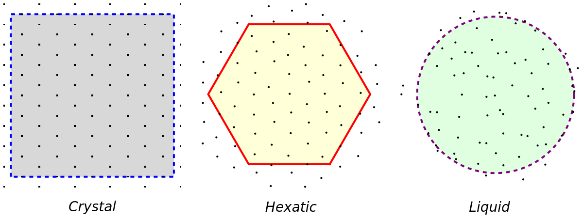
The picture below shows the three main kinds of order in 2D systems, namely crystalline, hexatic and liquid phases. In order to provide a quantitative description of the differences among them, one must consider the degree of translational (positional) and bond orientational order in the 2D point arrangements, whether it’s long range or short range. Translational order describes the regular repetition of points throughout the lattice: each lattice point can be mapped from a starting basis set by an integer number of translations. Bond orientational order takes into account how many nearest neighbors are found around each point and their average orientation with respect to a reference axis.
It is well known from condensed matter physics that crystalline systems exhibit both long-range translational and orientational, since it is a zero-entropy system.
On the opposite side, liquid order exhibits both short range translational and orientational order, therefore its entropy value is higher. During melting processes, according to the KTHNY theory of two-step melting, the long-range positional order is lost while bond-orientational order with sixfold symmetry is still retained, before being destroyed in the second step before the hexatic-to-liquid transition. This gives the so-called hexatic phase, which is an intermediate state of matter between the solid and the isotropic liquid phase, which contains also topological defects. For the development of KTHNY theory and the unbinding mechanism of defects, Kosterlitz and Thouless were awarded the 2016 Nobel Prize in Physics.
Getting the dataset
Getting the dataset
It' s rather straightforward to obtain a quick 2D graphical representation in Wolfram Language to simulate these three states of matter by adding random values to lattice coordinates and tuning the width range of the random uniform distribution in order to destroy gradually the lattice periodicity . As shown in the central graphics below, small perturbations applied to hexagonal lattice sites allow to simulate realistically hexatic systems with sixfold orientational order but short range positional order. By increasing the width of the RandomReal range a more disordered system with liquid - like features can be obtained . The shape of the simulation box (square, hexagonal or circular) can be obtained by SpatialPointData from a 2D coordinate dataset applied to a chosen polygonal or circular region .
In[]:=
(*hexagonallatticebasis*)b={{-Sqrt[3],-1},{-Sqrt[3],1}}/2;(*Generatelatticepointsfromthebasis*)pts=Tuples[Range[-55,55],2].b;ptsstyle={Black,PointSize[0.25]};regions={Rectangle[{-4.5,-4.5},{4.5,4.5}],Disk[{0,0},5],RegularPolygon[{0,0},5,6]};GraphicsGrid[{{Show[{(*crystal*)Graphics[{LightGray,EdgeForm[Directive[Thick,Dashed,Blue]],Rectangle[{-4,-4},{4,4}]}],ListPlot[SpatialPointData[pts,regions[[1]]],Axes->False,PlotStyle->ptsstyle]}],Show[{(*hexatic-like*)Graphics[{LightYellow,EdgeForm[Directive[Thick,Red]],RegularPolygon[{0,0},4,6]}],ListPlot[SpatialPointData[pts+RandomReal[{-0.15,0.15},{Length[pts]}],regions[[2]]],Axes->False,PlotStyle->ptsstyle]}],Show[{(*liquid-like*)Graphics[{EdgeForm[Directive[Thick,Dashed,Purple]],LightGreen,Disk[{0,0},4.0]}],ListPlot[SpatialPointData[pts+RandomReal[{-0.5,0.5},{Length[pts]}],regions[[3]]],Axes->False,PlotStyle->ptsstyle]}]},{Column[{Spacer[10],Style["Crystal",Black,Italic,14],Spacer[20]}],Column[{Spacer[10],Style["Hexatic",Black,Italic,14],Spacer[20]}],Column[{Spacer[10],Style["Liquid",Black,Italic,14],Spacer[20]}]}}]
Out[]=
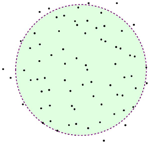
To obtain realistic dataset one must resort to the output configurations of molecular dynamics simulations, often based on Lennard-Jones interaction potentials between rods, disks or other systems. Sometimes, one could be interested into reproducing results from older papers from which datasets are not available. Wolfram Language can provide us with all the tools to get automatically point coordinates from imported images. The code in this post can be very useful if points are well apart from each other and distinguishable. Here is a slightly modified version applied to a static image. The user needs first to adjust the parameter in Binarize function and the chosen color matching the points of interest, in order to exclude other image details such as edges of different color.
The processingPipeline liner code allows the black points to be very well matched by the crosses provided by ImageMarker
The processingPipeline liner code allows the black points to be very well matched by the crosses provided by ImageMarker
In[]:=
imgliq=
;processingPipeline=Composition[HighlightImage[imgliq,ImageMarker[#,"Cross"]]&,#[[All,2]]&,ComponentMeasurements[#,"Centroid"]&,Binarize[#,0.4]&,ImageAdjust,DistanceTransform,Binarize,ColorDetect[#,Black]&];processingPipeline[imgliq]
Out[]=
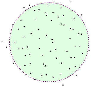
After adjusting options, the following code allows to get straightforwardly the point coordinates for further analysis.
In[]:=
processingPipelineData=Composition[#[[All,2]]&,ComponentMeasurements[#,"Centroid"]&,Binarize[#,0.4]&,ImageAdjust,DistanceTransform,Binarize,ColorDetect[#,Black]&];liqdata=processingPipelineData[imgliq]
Out[]=
{{354.5,564.},{467.5,564.},{313.,546.5},{196.,542.5},{158.5,529.},{405.,525.5},{256.567,514.1},{226.5,507.5},{349.618,493.618},{300.,492.},{535.45,477.4},{308.5,476.5},{417.853,472.5},{385.853,464.5},{487.5,453.},{236.,452.},{138.4,443.45},{341.,443.5},{405.,418.5},{83.,412.},{421.5,411.},{159.346,398.731},{464.5,388.5},{120.5,383.786},{482.269,382.346},{252.5,379.5},{205.5,356.},{520.,355.},{539.,350.5},{306.214,343.5},{157.5,332.},{260.,321.5},{461.289,320.5},{343.6,315.45},{585.,307.},{12.5,300.},{349.,297.5},{96.5,295.},{526.,272.},{497.567,266.9},{42.5,265.},{179.,264.5},{149.5,259.},{123.,256.},{259.45,255.4},{365.382,248.5},{587.,243.5},{331.,237.5},{441.5,235.5},{542.857,223.286},{196.5,216.5},{281.5,212.5},{166.389,210.444},{469.,197.5},{489.857,194.571},{374.1,191.433},{91.5,159.},{406.143,158.286},{199.433,154.1},{287.563,152.25},{533.,148.},{164.5,143.},{298.,139.5},{495.5,135.},{457.,120.},{202.,91.5},{400.,87.},{171.447,84.7105},{304.813,80.625},{276.,76.},{501.5,75.5},{352.735,63.2647},{229.447,53.4474},{415.45,13.4}}
Voronoi Mesh Entropy vs Bond Orientational Order Parameter
Voronoi Mesh Entropy vs Bond Orientational Order Parameter
disLocate Mathematica package for measuring orientational order
disLocate Mathematica package for measuring orientational order
Order quantification from datasets of 2D self-assembled systems is nicely discussed in this paper, where the title itself refers actually to the accompanying Mathematica package disLocate. This package is available from this repository and works quite well also on the most recent versions of Mathematica, although its latest revision dates back to almost two years ago. The most interesting tool provided by disLocate package is the function BondOrderParameter, which provides a numerical estimation at each lattice site of the Bond Orientational Order Parameter (BOOP). Usually, the average BOOP value is reported to quantify and compare the degree of order in different hexatic systems. Historically, the first definition for the 2D hexatic order parameter was introduced by Nelson and Halperin in 1978 and later extend to 3D systems by J. P. Steinhardt in his 1983 paper [1, 2].
However, some shortcomings of the BOOP method of calculation have been discussed in recent papers, where some modifications to Steinhardt’s definition were reported and compared [3, 4]. Actually, the definition implemented in disLocate package is based on Delaunay triangulation.
Usage examples of BondOrderParameter applied to experimental dataset can be found in the related Supporting Information of disLocate package. Other interesting functions for condensed matter scientists provided by this package are plotting utilities of pair correlation functions and diffraction pattern from positions. Additionally, there is also the function Hexaticize which creates a hexatic lattice from a list of point positions perturbed by the standard deviation of a zero-mean normal distribution.
Wolfram Language Functions from Shannon entropy definition
Wolfram Language Functions from Shannon entropy definition
In this computational essay the author would like to introduce the definitions for the Shannon information entropy applied to Voronoi meshes and graphs as general tools for quantifying the degree of disorder in 2D systems. Such observables were introduced by E. Bormashenko and co-workers in Refs. [5, 6] and implemented by the author herself in functions MeshVoronoiEntropy and NearestNeighborGraphEntropy, respectively. Correspondingly, the Voronoi entropy of a mesh enables the quantification of the ordering of a 2D tessellated structure according to the Shannon information entropy definition =-ln where i is the number of polygon types, and is the fraction of polygons possessing n sides (edges) in a given Voronoi diagram, i . e . the coordination number of each polygon. On the same line, the entropy of a graph is defined as =-ln , where the probability =n()/E is given by the number of edges with length over the total number of edges . These functions allow to provide separate measurements for both orientational and translational order of a given set of 2D lattice points, while taking into account at the same time the weighted distribution of the nearest neighbor coordination number for each site. These functions may be also of general applicability also to datasets obtained from any given point processes. As a consequence, the author suggests to apply the term hexatic to 2D systems with strictly zero value of Voronoi mesh entropy, which corresponds to perfect bond orientational order, but non-zero value of graph Voronoi entropy corresponding to short-range positional order. All other systems with Voronoi mesh entropy greater than zero may be classified as belonging to the intermediate liquid-to-hexatic phase. The full documentation for MeshVoronoiEntropy and NearestNeighborGraphEntropy is available from the matching webpages on Wolfram Function Repository (see here link).
S
vor
Σ
i
P
i
P
i
P
i
graph
S
Σ
i
P
L
i
P
L
i
P
L
i
L
i
L
i
E
Examples
Examples
General usage and basic results
General usage and basic results
First, let’s obtain the point coordinates and generate the associated mesh region and nearest neighbor graph for a crystalline structure:
In[]:=
crystpts=First@First@SpatialPointData[pts,regions[[1]]];meshvorcryst=VoronoiMesh[crystpts];regcryst=MeshRegion[MeshCoordinates[meshvorcryst],With[{a=PropertyValue[{meshvorcryst,2},MeshCellMeasure]},With[{m=1},Pick[MeshCells[meshvorcryst,2],UnitStep[a-m],0]]],MeshCellLabel{2"Index"}];graphcryst=NearestNeighborGraph[crystpts,{All,1.0}];
In[]:=
GraphicsRow[{Show[regcryst,{ImageSize->200}],Show[graphcryst,{ImageSize->200}]}]
Out[]=
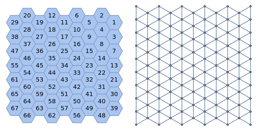
In[]:=
RowStyle["Mesh Voronoi Entropy: "],StyleToExpression@[regcryst],Spacer[20],Style["Graph Voronoi Entropy: "],Style[crystpts,1.0]
Out[]=
Mesh Voronoi Entropy: 0.
Graph Voronoi Entropy: 0

Now, let’s obtain the corresponding results for a hexatic structure:
In[]:=
hexaticpts=First@First@SpatialPointData[pts+RandomReal[{-0.01,0.01},{Length[pts]}],regions[[2]]];meshvorhexatic=VoronoiMesh[hexaticpts];reghexatic=MeshRegion[MeshCoordinates[meshvorhexatic],With[{a=PropertyValue[{meshvorhexatic,2},MeshCellMeasure]},With[{m=1},Pick[MeshCells[meshvorhexatic,2],UnitStep[a-m],0]]],MeshCellLabel{2"Index"}];graphhexatic=NearestNeighborGraph[hexaticpts,{All,1.2}];
In[]:=
GraphicsRow[{Show[reghexatic,{ImageSize->200}],Show[graphhexatic,{ImageSize->200}]}]
Out[]=
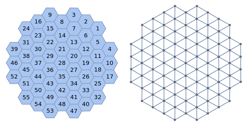
Finally, let’s increase disorder to obtain both non-zero mesh and graph Voronoi entropy for a liquid structure:
Applications to the computation of Voronoi mesh entropy for graphene dislocation defects
Applications to the computation of Voronoi mesh entropy for graphene dislocation defects
Without resorting to ab-initio calculations which require specialized packages with often steep learning curves, one can compute the disorder related to different 2D dislocation defects in graphene lattice (a pentagon, a heptagon and adjacent and separated heptagon-pentagon pairs) by a quicker estimate of mesh Voronoi entropy with the help of author contributed function MeshVoronoiEntropy.
In the following code, the atomic coordinates of a 2D system are converted to an undirected planar graph with NearestNeighborGraph; with the help of PlanarFaceList the graph is then represented as MeshRegion, which can be fed as input to MeshVoronoiEntropy function.
In the following code, the atomic coordinates of a 2D system are converted to an undirected planar graph with NearestNeighborGraph; with the help of PlanarFaceList the graph is then represented as MeshRegion, which can be fed as input to MeshVoronoiEntropy function.
For more complex dislocation defects the input distance entry in the NearestNeighborGraph function appearing in the Module code needs to be properly set to 80, in order to avoid multiple edge crossing in the resulting planar graph. For instance, for either separated or adjacent heptagon-pentagon pairs one gets
Interestingly, one can notice a decrease in mesh Voronoi entropy when the pentagon and heptagon are not adjacent.
Application to 2D quasicrystals: the Penrose tilings
Application to 2D quasicrystals: the Penrose tilings
In the following some planar graphs corresponding to different realizations of the Penrose tiling are reported. The vertex connections and site coordinates with 11, 31 and 86 elements were copied from this link.
These planar graphs can be converted into their corresponding mesh regions with the following function
It’s rather straightforward to check that both Voronoi mesh entropy and graph entropy are exactly zero for Penrose tiles. In this case, a slightly modified version of the code used in NearestNeighborGraphEntropy is used in order to work with planar graphs.
This is not the case with 2D Fibonacci quasicrystals, as shown in the example documentation of NearestNeighborGraphEntropy as their graph edges are unequal.
Summary
Summary
In this post several user-contributed function utilities have been presented, which can be helpful for condensed-matter scientists to quantify order in different 2D systems; the shown examples may be especially useful when teaching phase transitions and order classification in low-dimensional systems. The use of Voronoi graph and mesh entropy, which are based on the information theory entropy definition provided by Shannon are rather straightforward to implement and easier to be used since they only require site coordinates as input to their function implementation.
References
References
[1] Nelson D. and Halperin B., Phys . Rev . B 19, 2457 (1979)., “Dislocation-mediated melting in two dimensions”, https://doi.org/10.1103/PhysRevB.19.2457
[2] Steinhardt P., Nelson D., and Ronchetti M., Phys . Rev . B 28, 784 (1983).,”Bond-orientational order in liquids and glasses”, https://doi.org/10.1103/PhysRevB.28.784
[4] Haeberle J., Sperle M., and Born P., “Distinguishing noisy crystalline structures using bond orientational order parameters”, Eur. Phys. J. E42, 149 (2019). https://doi.org/10.1140/epje/i2019-11915-7
[5] Frenkel M., Legchenkova I., Shvalb N., Shoval S. and Bormashenko E., “Voronoi Diagrams Generated by the Archimedes Spiral: Fibonacci Numbers, Chirality and Aesthetic Appeal.”, Symmetry, 2023, no. 15, 746, 2023. https://doi.org/10.3390/sym15030746
CITE THIS NOTEBOOK
CITE THIS NOTEBOOK
Some utilities for order quantification in 2D disordered systems
by Jessica Alfonsi
Wolfram Community, STAFF PICKS, February 24, 2025
https://community.wolfram.com/groups/-/m/t/3399949
by Jessica Alfonsi
Wolfram Community, STAFF PICKS, February 24, 2025
https://community.wolfram.com/groups/-/m/t/3399949