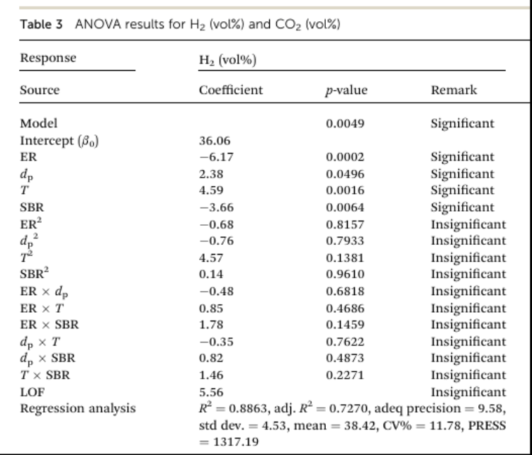
RSM is performed for the gasification of eucalyptus wood sawdust. We plot the Pareto chart. This chart indicates that only x1, x2, x3 and x4 are significant in agreement with the conclusions reported in Ref. 1
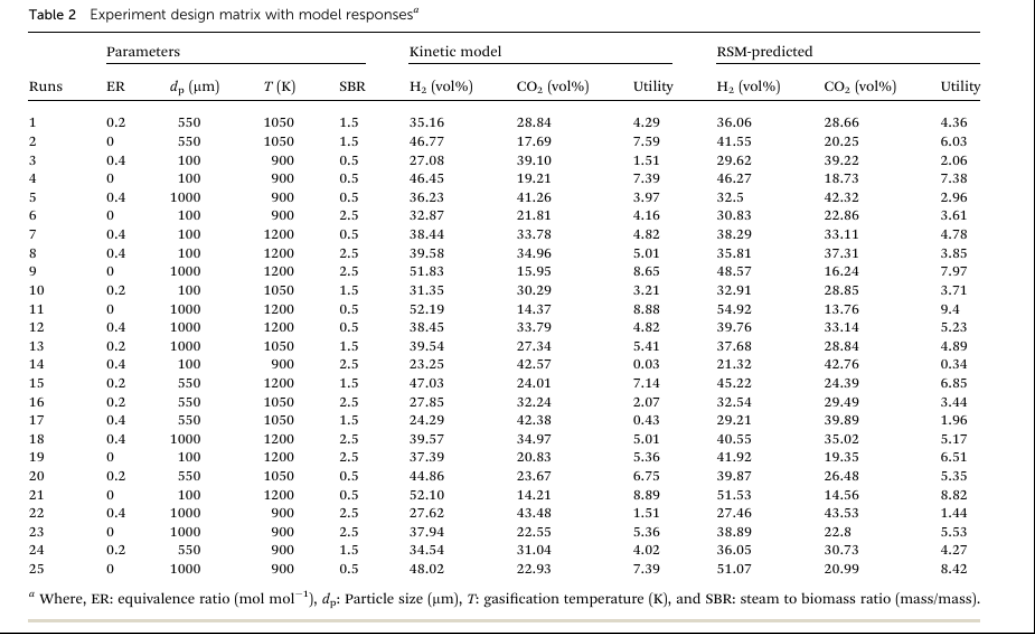
Experiment design matrix with model responses
In[]:=
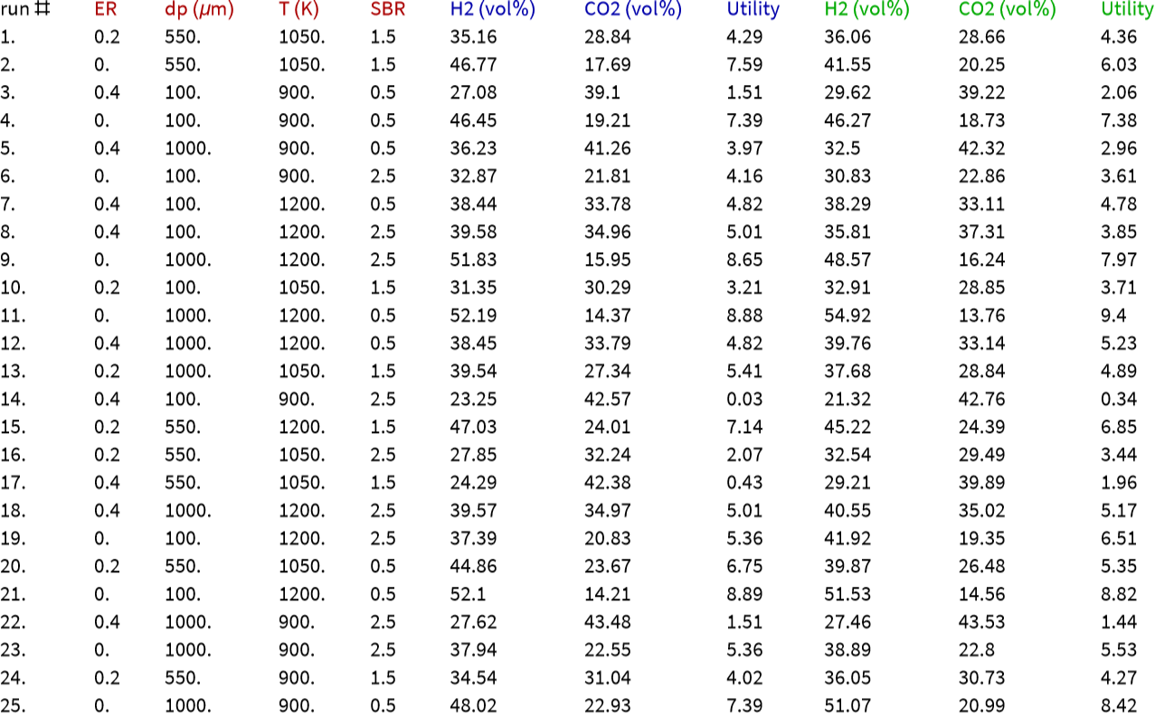
tbl=Join[{{"run #",Style["ER",Darker@Red],Style["dp (μm)",Darker@Red],Style["T (K)",Darker@Red],Style["SBR",Darker@Red],Style["H2 (vol%) ",Darker@Blue],Style["CO2 (vol%)",Darker@Blue],Style["Utility",Darker@Blue],Style["H2 (vol%) ",Darker@Green],Style["CO2 (vol%)",Darker@Green],Style["Utility",Darker@Green]}},{{1.,0.2,550.,1050.,1.5,35.16,28.84,4.29,36.06,28.66,4.36},{2.,0.,550.,1050.,1.5,46.77,17.69,7.59,41.55,20.25,6.03},{3.,0.4,100.,900.,0.5,27.08,39.10,1.51,29.62,39.22,2.06},{4.,0.,100.,900.,0.5,46.45,19.21,7.39,46.27,18.73,7.38},{5.,0.4,1000.,900.,0.5,36.23,41.26,3.97,32.5,42.32,2.96},{6.,0.,100.,900.,2.5,32.87,21.81,4.16,30.83,22.86,3.61},{7.,0.4,100.,1200.,0.5,38.44,33.78,4.82,38.29,33.11,4.78},{8.,0.4,100.,1200.,2.5,39.58,34.96,5.01,35.81,37.31,3.85},{9.,0.,1000.,1200.,2.5,51.83,15.95,8.65,48.57,16.24,7.97},{10.,0.2,100.,1050.,1.5,31.35,30.29,3.21,32.91,28.85,3.71},{11.,0.,1000.,1200.,0.5,52.19,14.37,8.88,54.92,13.76,9.4},{12.,0.4,1000.,1200.,0.5,38.45,33.79,4.82,39.76,33.14,5.23},{13.,0.2,1000.,1050.,1.5,39.54,27.34,5.41,37.68,28.84,4.89},{14.,0.4,100.,900.,2.5,23.25,42.57,0.03,21.32,42.76,0.34},{15.,0.2,550.,1200.,1.5,47.03,24.01,7.14,45.22,24.39,6.85},{16.,0.2,550.,1050.,2.5,27.85,32.24,2.07,32.54,29.49,3.44},{17.,0.4,550.,1050.,1.5,24.29,42.38,0.43,29.21,39.89,1.96},{18.,0.4,1000.,1200.,2.5,39.57,34.97,5.01,40.55,35.02,5.17},{19.,0.,100.,1200.,2.5,37.39,20.83,5.36,41.92,19.35,6.51},{20.,0.2,550.,1050.,0.5,44.86,23.67,6.75,39.87,26.48,5.35},{21.,0.,100.,1200.,0.5,52.10,14.21,8.89,51.53,14.56,8.82},{22.,0.4,1000.,900.,2.5,27.62,43.48,1.51,27.46,43.53,1.44},{23.,0.,1000.,900.,2.5,37.94,22.55,5.36,38.89,22.8,5.53},{24.,0.2,550.,900.,1.5,34.54,31.04,4.02,36.05,30.73,4.27},{25.,0.,1000.,900.,0.5,48.02,22.93,7.39,51.07,20.99,8.42}}];
In[]:=
tbl//TableForm
Out[]//TableForm=
In[]:=
low={0,100,900,0.5};high={0.4,1000,1200,2.5};
In[]:=
mid=0.5(low+high)
Out[]=
{0.2,550.,1050.,1.5}
In[]:=
halfrange=0.5(high-low)
Out[]=
{0.2,450.,150.,1.}
In[]:=
codedvar=Table[(tbl[[i,j+1]]-mid[[j]])/halfrange[[j]],{i,2,26},{j,1,4}]
Out[]=
{{0.,0.,0.,0.},{-1.,0.,0.,0.},{1.,-1.,-1.,-1.},{-1.,-1.,-1.,-1.},{1.,1.,-1.,-1.},{-1.,-1.,-1.,1.},{1.,-1.,1.,-1.},{1.,-1.,1.,1.},{-1.,1.,1.,1.},{0.,-1.,0.,0.},{-1.,1.,1.,-1.},{1.,1.,1.,-1.},{0.,1.,0.,0.},{1.,-1.,-1.,1.},{0.,0.,1.,0.},{0.,0.,0.,1.},{1.,0.,0.,0.},{1.,1.,1.,1.},{-1.,-1.,1.,1.},{0.,0.,0.,-1.},{-1.,-1.,1.,-1.},{1.,1.,-1.,1.},{-1.,1.,-1.,1.},{0.,0.,-1.,0.},{-1.,1.,-1.,-1.}}
Coded variables (The central composite design (CCD) technique is employed to conduct the optimization analysis).
In[]:=
codedvar//TableForm
Out[]//TableForm=
0. | 0. | 0. | 0. |
-1. | 0. | 0. | 0. |
1. | -1. | -1. | -1. |
-1. | -1. | -1. | -1. |
1. | 1. | -1. | -1. |
-1. | -1. | -1. | 1. |
1. | -1. | 1. | -1. |
1. | -1. | 1. | 1. |
-1. | 1. | 1. | 1. |
0. | -1. | 0. | 0. |
-1. | 1. | 1. | -1. |
1. | 1. | 1. | -1. |
0. | 1. | 0. | 0. |
1. | -1. | -1. | 1. |
0. | 0. | 1. | 0. |
0. | 0. | 0. | 1. |
1. | 0. | 0. | 0. |
1. | 1. | 1. | 1. |
-1. | -1. | 1. | 1. |
0. | 0. | 0. | -1. |
-1. | -1. | 1. | -1. |
1. | 1. | -1. | 1. |
-1. | 1. | -1. | 1. |
0. | 0. | -1. | 0. |
-1. | 1. | -1. | -1. |
Forming MD (the Computation Matrix)
In[]:=
M=codedvar;
In[]:=
x1=Transpose[M][[1]]
Out[]=
{0.,-1.,1.,-1.,1.,-1.,1.,1.,-1.,0.,-1.,1.,0.,1.,0.,0.,1.,1.,-1.,0.,-1.,1.,-1.,0.,-1.}
In[]:=
Dimensions[x1]
Out[]=
{25}
In[]:=
x2=Transpose[M][[2]]
Out[]=
{0.,0.,-1.,-1.,1.,-1.,-1.,-1.,1.,-1.,1.,1.,1.,-1.,0.,0.,0.,1.,-1.,0.,-1.,1.,1.,0.,1.}
In[]:=
x3=Transpose[M][[3]]
Out[]=
{0.,0.,-1.,-1.,-1.,-1.,1.,1.,1.,0.,1.,1.,0.,-1.,1.,0.,0.,1.,1.,0.,1.,-1.,-1.,-1.,-1.}
In[]:=
x4=Transpose[M][[4]]
Out[]=
{0.,0.,-1.,-1.,-1.,1.,-1.,1.,1.,0.,-1.,-1.,0.,1.,0.,1.,0.,1.,1.,-1.,-1.,1.,1.,0.,-1.}
In[]:=
MD=Transpose[{Table[1.0,{i,1,25}],x1,x2,x3,x4,x1x1,x2x2,x3x3,x4x4,x1x2,x1x3,x1x4,x2x3,x2x4,x3x4}];
In[]:=
Dimensions[MD]
Out[]=
{25,15}
In[]:=
Grid[MD,Frame->All]
Out[]=
1. | 0. | 0. | 0. | 0. | 0. | 0. | 0. | 0. | 0. | 0. | 0. | 0. | 0. | 0. |
1. | -1. | 0. | 0. | 0. | 1. | 0. | 0. | 0. | 0. | 0. | 0. | 0. | 0. | 0. |
1. | 1. | -1. | -1. | -1. | 1. | 1. | 1. | 1. | -1. | -1. | -1. | 1. | 1. | 1. |
1. | -1. | -1. | -1. | -1. | 1. | 1. | 1. | 1. | 1. | 1. | 1. | 1. | 1. | 1. |
1. | 1. | 1. | -1. | -1. | 1. | 1. | 1. | 1. | 1. | -1. | -1. | -1. | -1. | 1. |
1. | -1. | -1. | -1. | 1. | 1. | 1. | 1. | 1. | 1. | 1. | -1. | 1. | -1. | -1. |
1. | 1. | -1. | 1. | -1. | 1. | 1. | 1. | 1. | -1. | 1. | -1. | -1. | 1. | -1. |
1. | 1. | -1. | 1. | 1. | 1. | 1. | 1. | 1. | -1. | 1. | 1. | -1. | -1. | 1. |
1. | -1. | 1. | 1. | 1. | 1. | 1. | 1. | 1. | -1. | -1. | -1. | 1. | 1. | 1. |
1. | 0. | -1. | 0. | 0. | 0. | 1. | 0. | 0. | 0. | 0. | 0. | 0. | 0. | 0. |
1. | -1. | 1. | 1. | -1. | 1. | 1. | 1. | 1. | -1. | -1. | 1. | 1. | -1. | -1. |
1. | 1. | 1. | 1. | -1. | 1. | 1. | 1. | 1. | 1. | 1. | -1. | 1. | -1. | -1. |
1. | 0. | 1. | 0. | 0. | 0. | 1. | 0. | 0. | 0. | 0. | 0. | 0. | 0. | 0. |
1. | 1. | -1. | -1. | 1. | 1. | 1. | 1. | 1. | -1. | -1. | 1. | 1. | -1. | -1. |
1. | 0. | 0. | 1. | 0. | 0. | 0. | 1. | 0. | 0. | 0. | 0. | 0. | 0. | 0. |
1. | 0. | 0. | 0. | 1. | 0. | 0. | 0. | 1. | 0. | 0. | 0. | 0. | 0. | 0. |
1. | 1. | 0. | 0. | 0. | 1. | 0. | 0. | 0. | 0. | 0. | 0. | 0. | 0. | 0. |
1. | 1. | 1. | 1. | 1. | 1. | 1. | 1. | 1. | 1. | 1. | 1. | 1. | 1. | 1. |
1. | -1. | -1. | 1. | 1. | 1. | 1. | 1. | 1. | 1. | -1. | -1. | -1. | -1. | 1. |
1. | 0. | 0. | 0. | -1. | 0. | 0. | 0. | 1. | 0. | 0. | 0. | 0. | 0. | 0. |
1. | -1. | -1. | 1. | -1. | 1. | 1. | 1. | 1. | 1. | -1. | 1. | -1. | 1. | -1. |
1. | 1. | 1. | -1. | 1. | 1. | 1. | 1. | 1. | 1. | -1. | 1. | -1. | 1. | -1. |
1. | -1. | 1. | -1. | 1. | 1. | 1. | 1. | 1. | -1. | 1. | -1. | -1. | 1. | -1. |
1. | 0. | 0. | -1. | 0. | 0. | 0. | 1. | 0. | 0. | 0. | 0. | 0. | 0. | 0. |
1. | -1. | 1. | -1. | -1. | 1. | 1. | 1. | 1. | -1. | 1. | 1. | -1. | -1. | 1. |
H2 (vol %)
Using LinearModelFit to get the model
Statistical and ANOVA analyses
Statistical and ANOVA analyses
A small p - value (typically < 0.05) means the variable significantly contributes to explaining the outcome . A large p - value suggests the variable may not be important in the model and should be dropped from the model equation .
Predicted responses
Pareto Chart of Standardized Effects with significance threshold (dotted red line).
This chart confirms that only x1, x2, x3 and x4 are significant.
This chart confirms that only x1, x2, x3 and x4 are significant.
References
References
◼
[1] A. Sharma and R. Nath, H2-rich syngas production from gasification involving kinetic modeling: RSM-utility optimization and techno-economic analysis, RSC Adv., 13 (15) 2023, pp. 10308-10321, DOI: https://doi.org/10.1039/D3RA00287J
CITE THIS NOTEBOOK
CITE THIS NOTEBOOK
Pareto chart for gasification of eucalyptus wood sawdust
by Housam Binous and Ahmed Bellagi
Wolfram Community, STAFF PICKS, November 13, 2025
https://community.wolfram.com/groups/-/m/t/3574355
by Housam Binous and Ahmed Bellagi
Wolfram Community, STAFF PICKS, November 13, 2025
https://community.wolfram.com/groups/-/m/t/3574355