ORIGINAL ARTICLE: Dorst, Kevin (2024), Bayesians Commit the Gambler’s Fallacy. SSRN: http://dx.doi.org/10.2139/ssrn.4683064
SUBSTACK POST
SUBSTACK POST
Article Abstract: The gambler’s fallacy is the tendency to expect random processes to switch more often than they actually do—for example, to think that after a string of tails, a heads is more likely. It’s often taken to be evidence for irrationality. It isn’t. Rather, it’s to be expected from a group of Bayesians who begin with causal uncertainty, and then observe unbiased data from an (in fact) statistically independent process. Although they converge toward the truth, they do so in an asymmetric way—ruling out “streaky” hypotheses more quickly than “switchy” ones. As a result, the majority (and the average) exhibit the gambler’s fallacy. If they have limited memory, this tendency persists even with arbitrarily-large amounts of data. Indeed, such Bayesians exhibit a variety of the empirical trends found in studies of the gambler’s fallacy: they expect switches after short streaks but continuations after long ones; these nonlinear expectations vary with their familiarity with the causal system; their predictions depend on the sequence they’ve just seen; they produce sequences that are too switchy; and they exhibit greater rates of gambler’s reasoning when forming binary predictions than when forming probability estimates. In short: what’s been thought to be evidence for irrationality may instead be rational responses to limited data and memory.
Introduction
Introduction
This notebook contains all code needed to generate results from the January 2024 version of “Bayesians Commit the Gambler’s Fallacy”. (Available at https://philpapers.org/rec/DORBCT.)
Please run the “Loading Functions (run this first!)” section before proceeding, as it will initialize all functions needed for the rest of the notebook.
The rest of this notebook follows the order of the paper. Most of the paper focuses on “streak chains”, wherein once a streak is broken the probabilities are set back to (near) 50% of each outcome. Later sections of the notebook show that the results are robust to variations, as discussed in the Objections section of the paper.
Some conventions:
1) I will use 1 for heads (or success) and 0 for tails (or failure) throughout. Sequences are lists, so the sequence HTHHT is represented {1,0,1,1,0}
2) In stochastic matrices of size N, I will use the first 1,2,...N/2 states to represent states in which the previous toss was a tails (0), and states N/2+1, N/2 + 2,..., N to represent states in which the previous toss was a heads (1). Thus the following represents an (streak) 2-step Switchy_70% process:
{{0.3,0,0.7,0},
{0.4,0,0.6,0},
{0,0.6,0,0.4},
{0,0.7,0,0.3}}
Label the four states in this chain 1,2,3, and 4 respectively. The chain is in state 1 when it has previously landed TT, in state 2 when it has landed HT, state 3 when it has landed TH, and state 4 when it has landed HH.
Initial states are randomly selected from the middle two—in this case, 2 and 3. Thus the sequence HTHHT, i.e. {1,0,1,1,0,0}, would:
- If initialized in state 2, take this chain through states {3,2,3,4,2,1}
- If initialized in state 3, take this chain through states {4,2,3,4,2,1}
Loading Functions (run this first!)
Loading Functions (run this first!)
Streak chains (“instant-fall chains”)
Streak chains (“instant-fall chains”)
Streak chains are the simple ones used throughout most of the notebook, in which once a streak is broken the probabilities instantly return to (near) 50% of each outcome. (I originally called them instant-fall chains, so that terminology is used at times this notebook, at least in function names). This section will introduce the code to generate all results involving Streak chains.
Generating chains and likelihoods
Generating chains and likelihoods
Limited data (full sequence): asymmetric closeness and convergence
Limited data (full sequence): asymmetric closeness and convergence
This subsection will provide the code to show that:
1) The Switchy likelihood distribution over full sequences is closer to the Steady one than the Sticky one is; and
2) As a result, Bayesians who start out uncertain and condition on a full sequence of outcomes will rule out Sticky more quickly than Switchy
We will work with 5-step chains that build up to 90% Switchy or Sticky:
In[]:=
(*GeneratingtheMarkovchainsforaSwitchy,Steady,andStickyprocesswith5steps*)MatrixForm[swi5=getChain[0.1,5]]MatrixForm[ste5=getChain[0.5,5]]MatrixForm[sti5=getChain[0.9,5]](*Calculatingthelikelihoodsforindividualoutcomesbasedonthechains*)getInstantPropLikelihoods[swi5PropLikes,swi5]getInstantPropLikelihoods[ste5PropLikes,ste5]getInstantPropLikelihoods[sti5PropLikes,sti5](*Calculatingthelikelihoodsforentiresequencesbasedonthechains*)getInstantSeqLikes[swi5SeqLikes,swi5]getInstantSeqLikes[ste5SeqLikes,ste5]getInstantSeqLikes[sti5SeqLikes,sti5]
Out[]//MatrixForm=
0.1 | 0 | 0 | 0 | 0 | 0.9 | 0 | 0 | 0 | 0 |
0.18 | 0 | 0 | 0 | 0 | 0.82 | 0 | 0 | 0 | 0 |
0 | 0.26 | 0 | 0 | 0 | 0.74 | 0 | 0 | 0 | 0 |
0 | 0 | 0.34 | 0 | 0 | 0.66 | 0 | 0 | 0 | 0 |
0 | 0 | 0 | 0.42 | 0 | 0.58 | 0 | 0 | 0 | 0 |
0 | 0 | 0 | 0 | 0.58 | 0 | 0.42 | 0 | 0 | 0 |
0 | 0 | 0 | 0 | 0.66 | 0 | 0 | 0.34 | 0 | 0 |
0 | 0 | 0 | 0 | 0.74 | 0 | 0 | 0 | 0.26 | 0 |
0 | 0 | 0 | 0 | 0.82 | 0 | 0 | 0 | 0 | 0.18 |
0 | 0 | 0 | 0 | 0.9 | 0 | 0 | 0 | 0 | 0.1 |
Out[]//MatrixForm=
0.5 | 0 | 0 | 0 | 0 | 0.5 | 0 | 0 | 0 | 0 |
0.5 | 0 | 0 | 0 | 0 | 0.5 | 0 | 0 | 0 | 0 |
0 | 0.5 | 0 | 0 | 0 | 0.5 | 0 | 0 | 0 | 0 |
0 | 0 | 0.5 | 0 | 0 | 0.5 | 0 | 0 | 0 | 0 |
0 | 0 | 0 | 0.5 | 0 | 0.5 | 0 | 0 | 0 | 0 |
0 | 0 | 0 | 0 | 0.5 | 0 | 0.5 | 0 | 0 | 0 |
0 | 0 | 0 | 0 | 0.5 | 0 | 0 | 0.5 | 0 | 0 |
0 | 0 | 0 | 0 | 0.5 | 0 | 0 | 0 | 0.5 | 0 |
0 | 0 | 0 | 0 | 0.5 | 0 | 0 | 0 | 0 | 0.5 |
0 | 0 | 0 | 0 | 0.5 | 0 | 0 | 0 | 0 | 0.5 |
Out[]//MatrixForm=
0.9 | 0 | 0 | 0 | 0 | 0.1 | 0 | 0 | 0 | 0 |
0.82 | 0 | 0 | 0 | 0 | 0.18 | 0 | 0 | 0 | 0 |
0 | 0.74 | 0 | 0 | 0 | 0.26 | 0 | 0 | 0 | 0 |
0 | 0 | 0.66 | 0 | 0 | 0.34 | 0 | 0 | 0 | 0 |
0 | 0 | 0 | 0.58 | 0 | 0.42 | 0 | 0 | 0 | 0 |
0 | 0 | 0 | 0 | 0.42 | 0 | 0.58 | 0 | 0 | 0 |
0 | 0 | 0 | 0 | 0.34 | 0 | 0 | 0.66 | 0 | 0 |
0 | 0 | 0 | 0 | 0.26 | 0 | 0 | 0 | 0.74 | 0 |
0 | 0 | 0 | 0 | 0.18 | 0 | 0 | 0 | 0 | 0.82 |
0 | 0 | 0 | 0 | 0.1 | 0 | 0 | 0 | 0 | 0.9 |
In[]:=
getInstantChain[0.9,4]
Out[]=
{{0.9,0,0,0,0.1,0,0,0},{0.8,0,0,0,0.2,0,0,0},{0,0.7,0,0,0.3,0,0,0},{0,0,0.6,0,0.4,0,0,0},{0,0,0,0.4,0,0.6,0,0},{0,0,0,0.3,0,0,0.7,0},{0,0,0,0.2,0,0,0,0.8},{0,0,0,0.1,0,0,0,0.9}}
Begin with (1).
We can start by visualizing the likelihood distributions over all possible sequences of a given length.
We can start by visualizing the likelihood distributions over all possible sequences of a given length.
In[]:=
(*Settingthesequencelengthandgeneratingallpossiblesequencesofthatlength*)seqLength=6;Length[allSeqs=Tuples[{0,1},seqLength]];(*Calculatingthesequencelikelihoodsforallsequencesforeachtypeofprocess*)listSwiSeqLikes=swi5SeqLikes[allSeqs[[#]]]&/@Range[Length[allSeqs]];listSteSeqLikes=ste5SeqLikes[allSeqs[[#]]]&/@Range[Length[allSeqs]];listStiSeqLikes=sti5SeqLikes[allSeqs[[#]]]&/@Range[Length[allSeqs]];(*Plottingthesequencelikelihoodsforthethreetypesofprocesses*)ListLinePlot[{listSwiSeqLikes,listSteSeqLikes,listStiSeqLikes},Filling->Axis,PlotMarkers->Automatic,PlotRange->Full,PlotLegends->{"Switchy","Steady","Sticky"},Frame->{True,True,False,False},FrameLabel->{"Sequence Number","Likelihood"}]
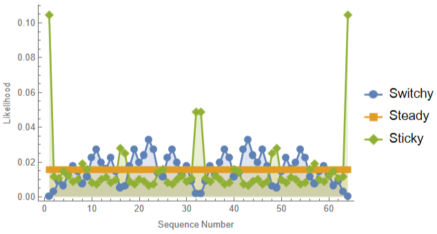
We can already see that Sticky has some big divergences from Steady, while Switchy seems to have less—(though this may be distorted by the linear scale, of course).
In[]:=
allSeqs[[1]]allSeqs[[32]]allSeqs[[33]]allSeqs[[64]]
Out[]=
{0,0,0,0,0,0}
Out[]=
{0,1,1,1,1,1}
Out[]=
{1,0,0,0,0,0}
Out[]=
{1,1,1,1,1,1}
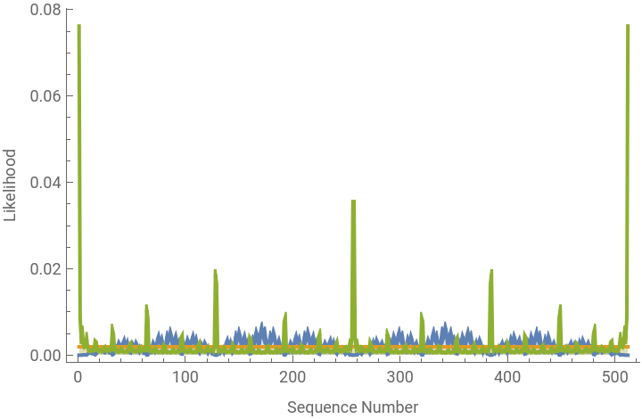
The divergence gets harder to see as we look at bigger sequences, where it can show up more, because the ordering is so unnatural:
In[]:=
(*Settingthesequencelengthandgeneratingallpossiblesequencesofthatlength*)seqLength=9;Length[allSeqs=Tuples[{0,1},seqLength]];(*Calculatingthesequencelikelihoodsforallsequencesforeachtypeofprocess*)listSwiSeqLikes=swi5SeqLikes[allSeqs[[#]]]&/@Range[Length[allSeqs]];listSteSeqLikes=ste5SeqLikes[allSeqs[[#]]]&/@Range[Length[allSeqs]];listStiSeqLikes=sti5SeqLikes[allSeqs[[#]]]&/@Range[Length[allSeqs]];(*Plottingthesequencelikelihoodsforthethreetypesofprocesses*)ListLinePlot[{listSwiSeqLikes,listSteSeqLikes,listStiSeqLikes},Filling->Axis,PlotRange->Full,PlotLegends->{"Switchy","Steady","Sticky"},Frame->{True,True,False,False},FrameLabel->{"Sequence Number","Likelihood"}]
Out[]=


This is slightly easier to see if we order the sequences in a relevant order, such as by the number of switches they contain:
In[]:=
(*Settingthesequencelength*)seqLength=9;(*Generatingallpossiblesequencesofheadsandtailswithalengthof10*)Length[allSeqs=Tuples[{0,1},seqLength]];(*Sortingthesequencesbasedonthenumberofswitchestheycontainusingthe'getNumSwitches'function*)allSeqs=SortBy[allSeqs,getNumSwitches];(*CalculatingthelikelihoodsofeachsortedsequencefortheSwitchyprocess*)listSwiSeqLikes=swi5SeqLikes[allSeqs[[#]]]&/@Range[Length[allSeqs]];(*CalculatingthelikelihoodsofeachsortedsequencefortheSteadyprocess*)listSteSeqLikes=ste5SeqLikes[allSeqs[[#]]]&/@Range[Length[allSeqs]];(*CalculatingthelikelihoodsofeachsortedsequencefortheStickyprocess*)listStiSeqLikes=sti5SeqLikes[allSeqs[[#]]]&/@Range[Length[allSeqs]];(*Plottingthesequencelikelihoodsforthethreeprocesses.Sequencesareorderedbytheirnumberofswitches.*)ListLinePlot[{listSwiSeqLikes,listSteSeqLikes,listStiSeqLikes},Filling->Axis,PlotRange->Full,ImageSize->Full(*PlotMarkers->Automatic*)(*Thislineiscommentedout;uncommenttoaddplotmarkers*)]
We can calculate the distances between these likelihood distributions with both the Euclidean and KL-Divergence measures:
The ratio of how much (Euclidean) farther Sticky is to Steady than Switchy is growing as the sequence-length grows:
Plot the Euclidean distances :
Note that though the difference is shrinking, the ratio is growing:
We can do the same with KL divergence, looking at the KL divergence from Steady to Switchy, compared to that from Steady to Sticky:
Initialize a list to store the KL divergences from Steady to Sticky/Switchy for various sequence lengths
Plot the KL Divergences
What this means is that, on average, if Bayesians start out unsure (say, uniform) between Switchy, Steady, and Sticky, and then observe a sequence of given length (seqLength) generated from a Steady process, their average probability for Sticky will fall faster than their average probability for Switchy.
We can simulate and visualize these averages with the following code:
(Note: this simulation takes awhile to run—about 1 -2 minutes on my machine. To exponentially speed it up, drop the length-100 or even length-50 sequences
(Note: this simulation takes awhile to run—about 1 -2 minutes on my machine. To exponentially speed it up, drop the length-100 or even length-50 sequences
First, get a list of various sequence lengths and the average posteriors in {Switchy, Steady, Sticky} upon conditioning on them :
Now visualize the trajectories at various sequence lengths :
Note that the ratio of mean posterior probability in Switchy to that in Sticky is growing:
Still, the fact that by the end of a 100-toss sequence people are so confident of Steady means that the degree to which they exhibit gambler’s or hot-hands reasoning will be fairly marginal.
For example, suppose we tell all our 10,000 Bayesians who’ve seen N-many tosses (for various N) that the coin has landed tails once in a row. This itself doesn’t provide evidence about whether the process is Switchy or Sticky, but it does tell them that if it’s Switchy, it’s 42% likely for the streak to continue—since then it’s in state 5 in the below Markov chain:
Similarly, if it’s Steady, it’s 50% likely to continue and if it’s Sticky, it’s 58% likely to continue.
Given this, we can calculate each agent’s credence in heads in the next toss by multiplying these likelihoods by their credences in the respective Switchy/Steady/Sticky hypotheses, and then plot the distribution of their credences in the next toss being heads.
For Bayesians that have only seen 20 tosses, there is quite a bit of variance:
For Bayesians that have only seen 20 tosses, there is quite a bit of variance:
But for those who’ve seen 100 tosses, they are almost all very close to 50%:
Those with mean credences after seeing 150 tosses, then seeing it land heads 3 times in a row:
Look at other test statistics:
Look at other test statistics:
We’ll simulate it, rather than calculate it.
Plot the three chain’ s likelihoods :
Plot the three chain’ s likelihoods:
Limited memory: asymmetric closeness and convergence
Limited memory: asymmetric closeness and convergence
As discussed in the paper [§___], I’ll use the unpacking model of limited memory. Given a sequence of 1000 tosses, the 1-unpacked memory of it records the total number of 1s; the 2-unpacked memory records both the number of 1s in the first half (500 tosses) and the number of 1s in the second half; and so on. Clearly the 1000-unpacked memory is the full sequence.
Begin by noting that now that we are focusing on proportions-of-1s, we can now visualize the sense in which the Steady likelihood distribution is closer to Switchy than to Sticky.
We can show this by looking at the likelihoods for the various possible numbers of 1s for various total numbers of outcomes, using our getInstantPropLikelihoods function from above:
Put likelihood functions in a list :
Plot likelihoods for various total tosses :
NOTES
1) the first time you run this, it’ ll take a few minutes, since swi5PropLikes and sti5PropLikes will needs to recursively calculate likelihoods out to 1000 tosses . Afterwards it’ ll run instantly (unless you Clear those functions) .
2) You will get a warning that precisino may be lost due to the small likkelihoods at the tails of the distribution . Don’ t worry about it——we’ ll virtually never sample from these tails anyways
Iterate through various numbers of tosses:
To verify this intuition, we can again plot Euclidean distances and KL divergences between Steady and Switchy/Sticky likelihoods as the number of tosses grows.
Euclidean distances:
Euclidean distances:
KL divergences:
KL divergences:
(NOTE: because of rounding errors (rounding small numbers down to 0), we can’t accurately calculate KL divergences for lengths greater than around 300; but the trend is clear)
Now we again plot the mean posteriors for agents who start out uniform over the process and condition on the memory-unpacked outcomes of 1000-toss sequences, for various depths of unpacking:
Create a list of simulations of Bayesians updating on the results of 1000 tosses, unpacked to various depths :
NOTE : unpacking of 1 is the hardest since this requires calculating likelihoods out to 1000 tosses . This takes a couple minutes on the first run, but will be instant afterward
The mean credence in a continuation after a streak of 2 and 3 with 20-unpacking are:
Mean ratios of posteriors in Switchy to Sticky:
Idea:
Idea:
Perhaps rounding errors? Let’s take the simPosts, translate into log odds, and then use to see whether the ratio is going up.
No, I don’t think that’s it. The numbers aren’t small enough to make Mathematica lose precision.
Maybe instead the average is misleading, because of the few people who are sky-high on Sticky?
What if we do the median instead?
Whoa, is this a difference between the limited-memory and limited data? For limited memory both the average and the median ratios are going way up. Check above.
Get log odds :
How to apply the logit function to every entry in simPosts[1], i.e. to the numbers inside each triple?

CITE THIS NOTEBOOK
CITE THIS NOTEBOOK
Bayesians Commit the Gambler's Fallacy
by Kevin Dorst
Wolfram Community, STAFF PICKS, January 25, 2024
https://community.wolfram.com/groups/-/m/t/3109698
by Kevin Dorst
Wolfram Community, STAFF PICKS, January 25, 2024
https://community.wolfram.com/groups/-/m/t/3109698