Top-down treadmill view at 90 km/h: the same car–trailer combination under three loading conditions — payload centre of mass 1.5 m ahead of the trailer axle (stable, green), exactly over the axle (marginal, amber), and 1.5 m behind it (unstable, red). All three start from the same 2.9° kick of the articulation angle θ. The animation is generated in Section 8 with swayAnimation[25.].
A linearised car–trailer model showing how payload position controls snaking instability via a Hopf bifurcation
A linearised car–trailer model showing how payload position controls snaking instability via a Hopf bifurcation
Anyone who has towed a trailer at highway speed knows the queasy feeling when the trailer starts swaying side to side. This snaking instability is not random buffeting — it is a Hopf bifurcation in the linearised yaw dynamics of the coupled car–trailer system. The single parameter that controls it is the position of the trailer’s centre of mass relative to its axle: load the weight ahead of the axle (high tongue weight) and the system is stable; load it behind the axle (low tongue weight) and lateral oscillations grow exponentially above a critical speed.
This notebook derives the 4-DOF linearised state-space model from first principles using Euler–Lagrange equations, writes out the full mass and force matrices, computes eigenvalues as a function of speed and payload position, identifies the Hopf bifurcation boundary in parameter space, and runs impulse-response simulations showing the stable, marginal, and unstable regimes. All code is in Wolfram Language using only built-in functions.
Audience: each section opens with an intuitive physical explanation, then deepens into a full mathematical treatment with equations and code. Vehicle dynamics researchers will recognise the linearised bicycle-model framework; general readers should be able to follow the physical narrative and see the bifurcation in the figures.
1. Setup
1. Setup
The notebook is self-contained: it needs only the package file TrailerSway.wl in the same folder. The package bundles the model (TrailerSway`TrailerModel`: state matrix, eigenvalues, impulse simulation) and the figure and animation functions (TrailerSway`TrailerPlots`). Every figure and the animation in this post is generated by the code cells below.
SetDirectory[NotebookDirectory[]];
Get["TrailerSway.wl"]
Get["TrailerSway.wl"]
As a first taste: the speed at which a moderately tail-heavy trailer (centre of mass 1 m behind the axle) goes unstable — in km/h:
Round[3.6 criticalSpeed[-1.]]
91
A typical highway speed. The rest of the post explains where this number comes from.
2. What is trailer sway?
2. What is trailer sway?
Trailer sway (also called snaking or fishtailing) is a lateral oscillation of a towed vehicle about the hitch point. Once initiated by a gust of wind, a lane change, or a bump in the road, the oscillation can either decay back to straight-line travel or grow until the driver loses control.
The phenomenon is dramatic and dangerous. Search YouTube for “trailer sway accident” and you will find hundreds of dashcam videos showing caravans, boat trailers, and utility trailers fishtailing violently at highway speed. A particularly instructive treadmill experiment by L2SFBC (Robert Pepper) demonstrates the effect using a 1/10-scale model car and trailer on a conveyor belt, with the payload moved to different positions on the trailer bed. The video (“Busting trailer weight distribution myths, demonstrated”, youtube.com/watch?v=JeEEC5eVNCk is an excellent visual companion to the mathematics that follows — and the animation at the top of this post is a simulated version of exactly that experiment.
The critical factor is tongue weight — the downward force that the trailer tongue exerts on the hitch ball. Tongue weight is determined by where the payload’s centre of mass sits relative to the trailer’s axle:
• High tongue weight (CoM ahead of axle, > 0): the system is stable at any realistic towing speed. After a perturbation, the lateral tire force on the trailer creates a restoring moment that damps the oscillation.
d
f
• Low / negative tongue weight (CoM behind axle, < 0): the same tire force creates an amplifying moment. Above a critical speed, small perturbations grow into large, dangerous oscillations.
d
f
For a single-axle trailer, statics links the two pictures: the tongue carries a vertical load =. With the parameters used below (m = 500 kg, = 3.5 m), = +0.5 m puts about 71 kgf on the hitch — 14% of the trailer’s weight, right in the classic 10–15% towing guidance — while = −1 m means the tongue pulls up on the hitch with about 143 kgf. Note that the yaw model below contains no vertical forces at all: enters purely as the geometric lever arm of the trailer tire force, and the cornering stiffnesses are held constant. Tongue weight is the everyday handle; is the parameter the mathematics actually sees.
W
tongue
mg
d
f
L
t
L
t
d
f
d
f
d
f
d
f
plotImpulseResponse[25., {{1.5, "Stable"}, {0., "Marginal"}, {-1.5, "Unstable"}}]
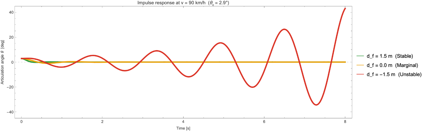
Figure 1. Impulse response of the articulation angle θ(t) at v = 90 km/h for three loading conditions: = +1.5 m (stable, green), 0 m (marginal, amber), −1.5 m (unstable, red).
d
f
3. The tongue-weight mechanism
3. The tongue-weight mechanism
Consider a single-axle trailer towed behind a vehicle at constant forward speed v. The trailer is connected to the tow vehicle at a ball hitch that allows free rotation in the yaw plane. The trailer has a single axle at distance behind the hitch.
L
t
When the trailer is displaced laterally (articulation angle θ ≠ 0), the trailer tire develops a lateral force proportional to its slip angle:
F
t
C
t
α
t
where is the tire cornering stiffness and is the slip angle at the trailer axle. The moment of this force about the hitch depends on where the trailer’s centre of mass is:
C
t
α
t
• If the CoM is ahead of the axle ( > 0), the tire force moment opposes the displacement — it is a restoring moment.
d
f
• If the CoM is behind the axle ( < 0), the tire force moment reinforces the displacement — it is an amplifying moment.
d
f
This sign change is the physical root of a Hopf bifurcation: as passes through a critical value (which depends on speed), a pair of complex-conjugate eigenvalues of the linearised system crosses the imaginary axis, and the equilibrium changes from a stable focus to an unstable focus. Below, we derive the full equations.
d
f
4. Mathematical model
4. Mathematical model
We use the linearised bicycle model (single-track model) for the tow vehicle coupled to a single-axle trailer through a free pivot at the hitch. The derivation proceeds in three steps: (i) define generalised coordinates and write the kinetic energy, (ii) compute the generalised forces from linear tire models, (iii) apply the Euler–Lagrange equations and transform to a first-order state-space form.
4.1 Generalised coordinates and geometry
4.1 Generalised coordinates and geometry
The generalised coordinates are:
• Y(t) — lateral displacement of the tow vehicle CoM from the nominal straight-line path.
• ψ(t) — vehicle yaw angle (heading).
• θ(t) — articulation angle, measured as the trailer’s heading relative to the vehicle’s heading.
The key geometric distances are:
• a = front axle to vehicle CoM, b = vehicle CoM to rear axle, h = rear axle to hitch. The total distance from vehicle CoM to hitch is c = b + h.
• = hitch to trailer axle, = distance from trailer CoM to trailer axle (positive = forward, toward hitch), e = − = distance from hitch to trailer CoM.
L
t
d
f
L
t
d
f
4.2 Kinetic energy and mass matrix
4.2 Kinetic energy and mass matrix
In the ground frame, linearised for small angles, the hitch sits a distance c behind the vehicle CoM, so its lateral position is Y − cψ. The trailer CoM sits a further distance e behind the hitch along the trailer, whose absolute heading is ψ + θ; its lateral position is therefore Y − cψ − e(ψ + θ). The lateral velocities are:
Y
hitch
Y
ψ
Y
trailer
Y
ψ
ψ
θ
Y
ψ
θ
The kinetic energy of the system, including translational and rotational terms for both vehicle and trailer, is:
T=M++m+
1
2
2
Y
1
2
I
z
2
ψ
1
2
2
-(c+e)-e
Y
ψ
θ
1
2
I
t
2
+
ψ
θ
where M is the vehicle mass, m is the trailer mass, is the vehicle yaw inertia, and is the trailer yaw inertia about its own CoM. Expanding the squares and collecting terms gives a symmetric 3×3 mass matrix in the [Y, ψ, θ] coordinate system. The Euler–Lagrange equations are:
I
z
I
t
d
dt
∂T
∂
q
i
∂T
∂
q
i
Q
i
where the generalised forces come from the tire lateral forces (see §4.3).
Q
i
4.3 Tire forces and slip angles
4.3 Tire forces and slip angles
We use the linear tire model: the lateral force is proportional to the slip angle with cornering stiffness C:
F
y
The slip angle of a tire is the angle between the direction the tire points and the direction it actually travels. With the vehicle sideslip angle (the angle between the velocity vector and the heading) and the yaw rate, the slip angles at the three axles (front, rear, trailer), linearised for small angles, are:
β=/v-ψ
Y
r=
ψ
α
f
ar
v
Y
ψ
v
α
r
br
v
Y
ψ
v
α
t
(c+)r
L
t
v
L
t
θ
v
Y
L
t
ψ
L
t
θ
v
The trailer slip angle picks up three extra terms: the yaw lever arm c + from vehicle CoM to trailer axle, the articulation rate sweeping the axle sideways, and the articulation angle θ rotating the tire itself.
L
t
θ
4.4 State-space form
4.4 State-space form
The Euler–Lagrange equations in [Y, ψ, θ] still contain ψ explicitly (through the slip angles). Substituting =v(β+ψ) — the definition of the sideslip angle — makes ψ drop out entirely, so four states suffice:
Y
x=[β,r,θ,ω]whereβ=-ψ,r=,ω=
Y
v
ψ
θ
and the linearised equations of motion take the form:
M=Fx
x
The 4×4 mass matrix M, derived from the kinetic energy, is:
M=
(M+m)v | -m(c+e) | 0 | -me |
-m(c+e)v | I z 2 (c+e) I t | 0 | me(c+e)+ I t |
0 | 0 | 1 | 0 |
-mev | me(c+e)+ I t | 0 | I t 2 e |
The underlying 3×3 mass matrix in the original [Y, ψ, θ] coordinates is symmetric — a standard cross-check on any Lagrangian derivation. The 4×4 matrix above is not symmetric because the state transformation introduces factors of v in the first column (from =v(β+ψ)) and inserts the trivial row =ω. This is expected and correct.
Y
θ
The 4×4 force matrix F collects the tire-force terms and the inertial terms proportional to v r that arise when the ground-frame acceleration =v+r is split between the two sides of the equation:
..
Y
β
F=
- C s | -(M+m)v- C a v | C t | C t L t v |
-a C f C r L t C t | m(c+e)v- 2 a C f 2 b C r 2 (c+ L t C t v | -(c+ L t C t | -(c+ L t C t L t v |
0 | 0 | 0 | 1 |
L t C t | mev- L t C t L t v | - L t C t | - 2 L t C t v |
where the auxiliary stiffness sums are:
C
s
C
f
C
r
C
t
C
a
C
f
C
r
L
t
C
t
The state matrix is A = F, and stability is governed by its eigenvalues. The bifurcation parameter enters through e = − , which appears in both M and F.
-1
M
d
f
L
t
d
f
4.5 Parameter values
4.5 Parameter values
The default parameters used throughout this notebook are:
Tow vehicle: M = 1500 kg, = 2500 kg·, a = 1.1 m, b = 1.7 m, h = 0.8 m, = = 80 kN/radTrailer: m = 500 kg, = 500 kg·, = 3.5 m, = 60 kN/rad
I
z
2
m
C
f
C
r
I
t
2
m
L
t
C
t
These are representative of a mid-size SUV (1500 kg) towing a single-axle utility trailer (500 kg). The cornering stiffness values are typical for highway passenger tires.
4.6 Implementation
4.6 Implementation
The state matrix at 90 km/h with a well-loaded trailer ( = +1.5 m):
d
f
A = buildAMatrix[25., 1.5];
MatrixForm[A]
MatrixForm[A]
and its eigenvalues:
TableForm[{Re[#], Im[#]} & /@ Eigenvalues[A],
TableHeadings -> {None, {"Re(λ)", "Im(λ)"}}]
TableHeadings -> {None, {"Re(λ)", "Im(λ)"}}]
All real parts are negative — this configuration is stable at 90 km/h, as the well-damped impulse response in Figure 1 already showed.
5. Eigenvalue analysis and Hopf bifurcation
5. Eigenvalue analysis and Hopf bifurcation
5.1 Eigenvalue structure
5.1 Eigenvalue structure
Because A is 4×4 and real, the four eigenvalues come in complex-conjugate pairs or as real values. For the physically relevant parameter range, we typically find:
• One conjugate pair associated with the coupled yaw–articulation mode (the “trailer sway” mode). This is the mode whose real part crosses zero at the Hopf bifurcation.
• One conjugate pair (or two real eigenvalues) associated with the vehicle yaw mode, which is typically well-damped and does not participate in the instability.
plotMaxRealVsSpeed[{1.5, 0.5, 0., -0.5, -1.0, -1.5}]
5.2 The Hopf bifurcation
5.2 The Hopf bifurcation
A Hopf bifurcation occurs when a pair of complex-conjugate eigenvalues λ = σ ± iω crosses the imaginary axis, i.e., when σ = Re(λ) passes through zero while ω = Im(λ) ≠ 0. At the bifurcation point:
• For σ < 0 (before crossing): the equilibrium is a stable focus — perturbations spiral inward (damped oscillations).
• For σ > 0 (after crossing): the equilibrium is an unstable focus — perturbations spiral outward (growing oscillations).
• At the crossing (σ = 0): the system is marginally stable and oscillates at frequency ω.
Strictly speaking, a Hopf bifurcation is a property of the underlying nonlinear system: at the crossing, the nonlinear terms (here, tire saturation and finite-angle geometry, which the linearised model omits) determine the small limit cycle that is born. What the linear analysis establishes is exactly the ingredient the Hopf theorem requires of it — a complex-conjugate pair crossing the imaginary axis transversally with ω ≠ 0 while all other eigenvalues remain in the left half-plane.
plotEigenvalueLoci[{{1.5, "Stable"}, {0., "Marginal"}, {-1.5, "Unstable"}}]
Figure 3. Eigenvalue loci in the complex plane as speed increases from 30 to 160 km/h, for three loading conditions. In the unstable case the sway pair crosses into the right half-plane.
5.3 Bifurcation diagram
5.3 Bifurcation diagram
plotBifurcationDf[{20., 25., 30.}]
5.4 Critical speed
5.4 Critical speed
TableForm[
Table[{df, Module[{vc = criticalSpeed[df]},
If[vc === Infinity, "none found below 216 km/h",
Row[{Round[3.6 vc], " km/h"}]]]},
{df, {1.5, 0.5, 0., -0.5, -1., -1.5, -2.}}],
TableHeadings -> {None, {"d_f [m]", "critical speed"}}]
Table[{df, Module[{vc = criticalSpeed[df]},
If[vc === Infinity, "none found below 216 km/h",
Row[{Round[3.6 vc], " km/h"}]]]},
{df, {1.5, 0.5, 0., -0.5, -1., -1.5, -2.}}],
TableHeadings -> {None, {"d_f [m]", "critical speed"}}]
(216 km/h = 60 m/s is simply the ceiling of the default search range, chosen well beyond any legal towing speed — not a physical bound.)
6. Impulse response and phase portraits
6. Impulse response and phase portraits
To see the bifurcation in action, we integrate the state equations from an initial perturbation θ(0) = 0.05 rad ≈ 2.9° (all other states zero) at v = 90 km/h (25 m/s). This models a sudden small lateral disturbance — a gust of wind or a lane change. For the tail-heavy case:
sim = simulateImpulse[25., -1.5];
Plot[sim["theta"][t] 180/Pi, {t, 0, 8},
Frame -> True,
FrameLabel -> {{"θ [deg]", None}, {"Time [s]", None}},
PlotStyle -> Directive[Thickness[0.004], RGBColor[0.86, 0.20, 0.15]],
PlotLabel -> "Unstable trailer sway (d_f = -1.5 m)"]
Plot[sim["theta"][t] 180/Pi, {t, 0, 8},
Frame -> True,
FrameLabel -> {{"θ [deg]", None}, {"Time [s]", None}},
PlotStyle -> Directive[Thickness[0.004], RGBColor[0.86, 0.20, 0.15]],
PlotLabel -> "Unstable trailer sway (d_f = -1.5 m)"]
The three loading conditions show strikingly different behaviour:
plotPhasePortrait[25., {{1.5, "Stable"}, {0., "Marginal"}, {-1.5, "Unstable"}}]
plotImpulsePanel[25., -1.5]
Figure 6. Full state impulse response panel for the unstable case, showing all four state variables, the phase portrait, and the state energy xx growing exponentially.
7. The stability map
7. The stability map
plotStabilityMap[]
This is the quantitative version of the towing safety advice: always load heavy items over or ahead of the trailer axle. The stability map shows exactly how much margin you have, and how dramatically that margin shrinks with speed.
8. The treadmill animation
8. The treadmill animation
swayAnimation[25.]
The three regimes of Figure 1, rendered as motion: the stable trailer straightens out, the marginal one keeps swaying gently, and the tail-heavy one diverges until the linear model loses validity.
9. Conclusions
9. Conclusions
Key findings:
• The linearised model captures the essential physics: oscillation frequency (≈ 0.7 Hz), growth rate, and the critical speed are all in physically reasonable ranges.
• The 3×3 Lagrangian mass matrix in the original [Y, ψ, θ] coordinates is symmetric — a standard cross-check on the Euler–Lagrange derivation. The 4×4 state-space M is not symmetric due to the transformation to the sideslip state β, which is expected.
Model assumptions and limitations: the derivation is linear (small angles, linear tire forces), so it identifies the onset of instability, not the finite-amplitude sway that follows. Forward speed is held constant and the hitch is a frictionless pivot — hitch friction and friction dampers add damping and raise the critical speed (the subject of [5]). The cornering stiffnesses are held constant, so the redistribution of vertical axle loads that accompanies real tongue-weight changes is not modelled. And the specific critical speeds quoted are illustrative for the representative parameters of §4.5, not predictions for any particular vehicle.
The practical lesson is simple: tongue weight matters. Loading a trailer so that the centre of mass is well ahead of the axle is not optional — it is the difference between a stable and an unstable system at highway speed.
10. References
10. References
[1] Pacejka, H. B. (2012). Tire and Vehicle Dynamics, 3rd ed. Butterworth-Heinemann. ISBN 978-0-08-097016-5. [Standard reference for tire modelling and cornering stiffness.]
[2] Rajamani, R. (2012). Vehicle Dynamics and Control, 2nd ed. Springer. ISBN 978-1-4614-1432-2. [Chapter 2 derives the lateral bicycle model used here for the tow vehicle.]
[3] Deng, W. & Kang, X. (2003). “Parametric study on vehicle-trailer dynamics for stability control.” SAE Technical Paper 2003-01-1321. doi:10.4271/2003-01-1321. [Systematic parameter study of car–trailer stability with a similar linearised model; identifies trailer load position as the primary stability parameter.]
[4] Bundorf, R. T. (1967). “The influence of vehicle design parameters on characteristic speed and understeer.” SAE Technical Paper 670078. doi:10.4271/670078. [Early systematic study of vehicle directional stability.]
[5] Sharp, R. S. & Alonso Fernández, M. (2002). “Car–caravan snaking—Part 1: the influence of pintle pin friction.” Proceedings of the Institution of Mechanical Engineers, Part C: Journal of Mechanical Engineering Science 216(7), 707–722. doi:10.1243/09544060260128760. [Detailed analysis of caravan snaking instability including hitch friction and nonlinear effects.]
Experimental demonstrations: Pepper, R. (L2SFBC). “Busting trailer weight distribution myths, demonstrated.” YouTube, 2020. youtube.com/watch?v=JeEEC5eVNCk (https://www.youtube.com/watch?v=JeEEC5eVNCk). [Scale-model treadmill experiment showing the effect of payload position on trailer stability.] Also: Weigh Safe. Tongue weight treadmill demonstration. youtube.com/shorts/Fq19K682Wb8 (https://www.youtube.com/shorts/Fq19K682Wb8).
11. Reproducibility
11. Reproducibility
This notebook is fully runnable from the two files attached to the post: trailer_sway.nb and TrailerSway.wl. Put them in the same folder, open the notebook, and evaluate it top to bottom — every figure and the animation regenerate from the model.
All source code is also available at:
https://github.com/mthiel74/TrailerSway
To reproduce all figures and rebuild this notebook from scratch:
git clone https://github.com/mthiel74/TrailerSway.git
cd TrailerSway
# Standalone Wolfram figures
wolframscript -file wolfram/run_all.wls
# Rebuild this notebook (bundles TrailerSway.wl, evaluates all figures and the animation)
wolframscript -file community/build_notebook.wls
cd TrailerSway
# Standalone Wolfram figures
wolframscript -file wolfram/run_all.wls
# Rebuild this notebook (bundles TrailerSway.wl, evaluates all figures and the animation)
wolframscript -file community/build_notebook.wls
Generated on August 5, 2026 with Wolfram Language 15.0.
CITE THIS NOTEBOOK
CITE THIS NOTEBOOK
Trailer sway and the tongue-weight bifurcation
by Marco Thiel
Wolfram Community, STAFF PICKS, August 5, 2026
https://community.wolfram.com/groups/-/m/t/3774166
by Marco Thiel
Wolfram Community, STAFF PICKS, August 5, 2026
https://community.wolfram.com/groups/-/m/t/3774166