Cellular automata have the capability of forming many complex structures from simple underlying rules, giving insight into how it could model real life physical behavior. This project relates fundamental and non-fundamental elementary particles (electrons, quarks, protons, neutrons, etc.) found at a subatomic level to repetitive structures found in class 4 cellular automata. Using an AI algorithm, it effectively identifies these particles by looking at many evolutions from random initial conditions. It then displays the various results of their collisions considering different phase shifts on a scattering matrix (s-matrix) and an interactive multiway graph.
What are Class 4 Cellular Automata?
What are Class 4 Cellular Automata?
Since the 1940s, cellular automata (CA) have been a vital tool to model and simulate real-life situations in the scientific and non-scientific world. As per Wolfram's classification, cellular automata are partitioned into four classes.
◼
Class 1: All initial conditions lead to a uniform state.
◼
Class 2: All initial conditions lead to a repeating state.
◼
Class 3: Initial conditions lead to random behavior.
◼
Class 4: Initial conditions lead to many structures (subatomic particles in this case) that interact in many complicated ways.
This project will be focusing on the virtual particles within class 4 cellular automata. Amalgamating features from class 2 and class 3 cellular automata, these class 4 particles and their persistent structures are able to provide a simple model of the behavior of elementary particles (electrons, quarks, protons, neutrons, etc.). In Stephen Wolfram’s post earlier this year titled “On the Concept of (Wolfram, 2022), he describes the universe as containing “persistent structures” that are “carriers of pure motion.” He shows how these CA particles could act as a models of pure motion by continuing on their persistent paths and eventually interacting with other particles in the system. This project builds on that fact and analyzes how these structures behave and interact to give a better idea of the concept of motion in elementary particles and to give more insight to quantum behavior for future applications.
Motion”
Out[]=
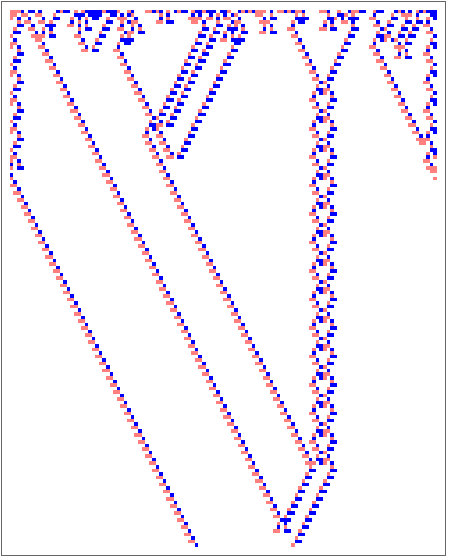
Example of class 4 cellular automata in rule 6,813,192,821,526.
Cellular Automata Definitions
Cellular Automata Definitions
In this study, I'll be using CA rule number 6,813,192,821,526 to analyze repeating subatomic particle structures along with their behaviors and collisions. Although each cell in elementary cellular automata (ECA) generally are defined as either black or white (1 or 0), I will be using a three way system for the cells (2, 1, 0) to depict the rule. Throughout the project, I'll be utilizing the definitions below to represent the situation and run my code. The following block creates a random initial condition and provides a visual representation of the particle behavior.
starting = RandomInteger[2,20]
Out[]=
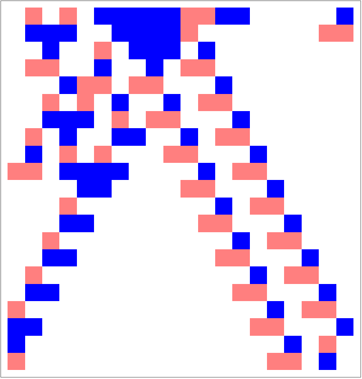
Here are the icons for the CA rule:
RulePlot[CellularAutomaton[{6813192821526, 3}], ColorRules->{2->Blue,1->Pink}]
Out[]=
Identifying the Particles
Identifying the Particles
I first started off by identifying the subatomic particles using the function findParticles—an AI algorithm. The function essentially breaks the matrix into submatrices and identifies repeating particle blocks in the grid. The algorithm then scans for submatrices that are surrounded by white cells, follow a straight line, and contain less than a certain number of white cells. I believe this is an optimal solution as it accounts for submatrices that could either be mostly white space, part of another bigger particle, or even part of a collision between other particles.
findParticles[2,2,starting,20]//Quiet
Out[]=
{{{1,0},{2,2}},{{0,2},{1,1}}}
Find particles of size sizeX and sizeY in cellular automata evolutions:
In[]:=
findParticles[sizeX_Integer, sizeY_Integer, startingList_List, length_Integer]:= Module[ {maxWhite = decideMaxWhite[sizeX, sizeY]}, counts = Select[Normal @ Counts @ Flatten[Partition[CellularAutomaton[{6813192821526, 3}, startingList, length], {sizeX,sizeY}, 1], 1], Length[Cases[#, 0, Infinity]] < maxWhite &]; Select[Keys[counts], trueParticleQ[sizeX, sizeY, startingList, #, length] &]]
The below function decides the maximum number of white cells available in the submatrix based on its size:
In[]:=
decideMaxWhite[sizeX_Integer, sizeY_Integer]:= If[(sizeX <= 4), 0.5 * sizeX * sizeY, 0.75 * sizeX * sizeY]
Given a submatrix of a certain size, this code block will find the number of true particles given the conditions stated above in my algorithm:
In[]:=
trueParticleQ[sizeX_Integer, sizeY_Integer, startingList_List, particle_List, length_Integer]:= Length[trueParticles[sizeX, sizeY, startingList, particle, length]] > 0trueParticles[sizeX_Integer, sizeY_Integer, startingList_List, particle_List, length_Integer]:= Module[ positions = Position[Partition[CellularAutomaton[{6813192821526, 3},startingList,length], {sizeX, sizeY}, 1], particle, Infinity], Select[positions, Length[possibleLines[positions]] > 0 && checkWhiteQ[#, length, sizeX, sizeY] &]]
checkWhiteQ verifies if the submatrix at a particular position is surrounded by white cells on the left and right:
In[]:=
checkWhiteQ[{x_Integer, y_Integer},length_Integer, sizeX_Integer, sizeY_Integer]:= AllTrue[Table[ca[[x + n, Mod[y - 1, length]]], {n, 0, sizeX - 1}], # == 0 &] && AllTrue[Table[ca[[x + n, Mod[y + sizeY, length]]], {n, 0, sizeX - 1}],# == 0 &]
possibleLines confirms if 4 or more particles lie on a straight line. This function will detect if the particle is moving to the right, left, or if it is stationary:
In[]:=
possibleLines[sizeX_Integer, sizeY_Integer, fullList_List]:= SequenceCases[fullList, {{a_, b_}, ___,{aa_, bb_}, ___,{aaa_, bbb_}, ___,{aaaa_, bbbb_}} /; (a + sizeX == aa & & b + 1== bb && a + sizeX * 2 == aaa && b + 2 == bbb && a + sizeX * 3 == aaaa && b + 3 == bbbb) || (a + sizeX == aa && b - 1 == bb && a + sizeX * 2 == aaa && b - 2 == bbb && a + sizeX * 3 == aaaa && b - 3 == bbbb) || (a + sizeX == aa && b == bb && a + sizeX * 2 == aaa && b == bbb && a + sizeX * 3 == aaaa && b == bbbb) :> {{a, b}, {aa, bb}, {aaa, bbb}, {aaaa, bbbb}}, Overlaps->True]
Identified Particles
Identified Particles
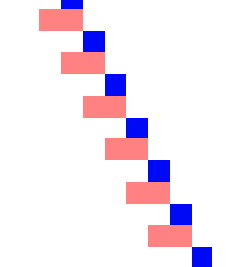
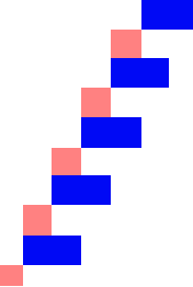
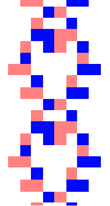
Running the particle detector through many initial conditions as well as manually looking through many combinations, I have identified 6 different particles: ,,B,,,D. I would consider and as fundamental particles considering that they are the building blocks of all the other particles (electrons, quarks, etc.). The + and - are used because they are structurally similar but move in opposite directions.
+
A
-
A
+
C
-
C
+
A
-
A
Particle Definitions
Particle Definitions
Out[]//TableForm=
+ A | - A |
Captured in a 2x2 submatrix. | Captured in a 2x2 submatrix. |
B: Particle with no velocity created by + A - A | |
Captured in a 8x8 submatrix. | |
Particle Interactions
Particle Interactions
As Wolfram mentioned, these particle structures never seem to move forever and instead they “always fairly quickly interact and ‘annihilate’” (Wolfram, 2022). The particles produced by this CA rule demonstrate these behaviors and due to the many different initial conditions that produce these particles, it is a given that they would have to interact. This observation gives more insight into motion and the quantum field theory about how objects in a particular system (on the subatomic level or greater) would end up interacting at some point.
To piece together Wolfram's analysis above, I created these particles and studied their motion and collision interactions. However, quite quickly I realized that these particles had different products based on how they collided. To account for this, I recorded all possible products based on all possible horizontal phase shifts and found a pattern in which they repeat periodically.
Collisions Create New Particles
Collisions Create New Particles
The below two pictures show particles creating new particles. The first one is a simple example of the two fundamental particles resulting in a more complex particle. This is the most common example since all non-fundamental particles are essentially combinations of these two fundamental particles (similar to how electrons, quarks, photons, etc. make up all other matter). Some of these fundamental particle collisions also have the ability to result in other fundamental particles as shown in the second picture. We are able to relate this to real life as two fundamental particles have the ability to create other fundamental particles just like how photons could create electrons by grazing past each other.
In the below two pictures, we can see different particles colliding to result in a combination of other particles (either fundamental particles or non-fundamental particles). Since all particles are bound to collide in such a system, we can see how new structures evolve and diverge in a certain period of time.
Collisions Annihilate the Particles
Collisions Annihilate the Particles
Visualizing Interactions
Visualizing Interactions
Scattering Matrix (S-Matrix)
Scattering Matrix (S-Matrix)
To visualize all particle interactions, the below s-matrix organizes the possible collisions containing the different products based on phase shifts. It is important to consider these phase shifts as the collisions behave differently based on the position at which they collide. The different possible products are separated by commas below.
Multiway Graph
Multiway Graph
As I was able to get different results from the same particles in a collision due to horizontal phase shifts, I was also able to create the following multiway graph to show the different results from these collisions. Multiway graphs show the different states a particular collision could go through at each evolution.
Conclusion and Future Directions
Conclusion and Future Directions
In conclusion, the results from above show how these particles identified in class 4 cellular automata have the ability to model elementary subatomic particles like electrons, protons, etc. From showing quantum behavior by being able to create new particles from fundamental particles to particle annihilation, this model consisting of simple persistent structures is able to provide a simple yet complex look into our universe and motion.
In the direction of code, I hope to improve the efficiency of the AI algorithm that detects particles by allowing it to detect particles in bigger grids in less time. To explore further in the topic, I would like to continue working on studying these particle interactions by creating Feynman diagrams to model these collisions more in detail. I would also like to see how you would be able to involve hypergraphs to study elementary particles in general and be able to model much more physical behavior and properties such as momentum, energy, and spin with the nodes, etc. Finally, I would also like to relate my findings to the quantum field theory and provide more insight into how such models are able to relate with the virtual particles discussed.
In the direction of code, I hope to improve the efficiency of the AI algorithm that detects particles by allowing it to detect particles in bigger grids in less time. To explore further in the topic, I would like to continue working on studying these particle interactions by creating Feynman diagrams to model these collisions more in detail. I would also like to see how you would be able to involve hypergraphs to study elementary particles in general and be able to model much more physical behavior and properties such as momentum, energy, and spin with the nodes, etc. Finally, I would also like to relate my findings to the quantum field theory and provide more insight into how such models are able to relate with the virtual particles discussed.
Citations and Credits
Citations and Credits
Special thanks to Stephen Wolfram for taking time out of his schedule to inspire, provide insight, and guide me through this project.
I would like to thank my mentor Peter Barendse and the rest of the Wolfram team for helping me out on the process of computational analysis. A big shout out to my family for always supporting and cheering me on through all my ventures.