Introduction
Introduction
In this notebook we present generalized Lanchester combat models and use one of them for simulation and calibration examples with data of the Battle of Iwo Jima.
Remark: The content of this notebook is intentionally theoretically fundamental, but short and simple both mathematically and code-wise. Author's intent is to develop similar computational workflows for (1) field battles, like the Normandy campaign during Word War II, 1944, or (2) urban warfare, like Second Battle of Fallujah, Iraq 2009, or Battle of Bakhmut, Ukraine 2023.
The main computational workflows are done with a System Dynamics (SD) software monad implemented in the paclet "MonadicSystemDynamics", [AAp2]. That paclet is based on the monad implementation presented in "A monad for Epidemiologic Compartmental Modeling Workflows", [AA1]. The functions provided by the paclet [AAp2] have the prefix "SDMon", which stands for "System Dynamics Monad".
Why use the Battle of Iwo Jima in examples?
Why use the Battle of Iwo Jima in examples?
The examples below use the Battle of Iwo Jima because that is convenient both data-wise and mathematics-wise. Here are our reasons:
◼
The battle is important for the USA military, hence well documented and used in multiple contexts.
◼
See, for example, mathematical articles like [JE1] and [RS1].
◼
(Relatively) well curated data can be found. Like:
◼
Sizes of the military forces
◼
Battle duration
◼
There is no need to:
◼
Take care of negative stocks
◼
Simulate "will to fight" -- Japanese soldiers fought to the last one
◼
Japanese Prisoners Of War (POWs) became POWs because they were found unconscious...
Notebook structure
Notebook structure
◼
Generalized model and variants
Main theory.
Main theory.
◼
SDMon Model
Programmer's version.
Programmer's version.
◼
Direct model simulation
Using the Battle of Iwo Jima data and related pre-computed rates.
Using the Battle of Iwo Jima data and related pre-computed rates.
◼
Calibration
We can get the theoretically computed rates by using numerics!
We can get the theoretically computed rates by using numerics!
◼
Future plans
Make models, not war.
Make models, not war.
Generalized models
Generalized models
This section presents a translation to English of introductory paragraphs of [NM1]. (The same general model and breakdown is presented in [AS1].)
In the most general form, the Lanchester models can be described by the by the equation:
In[]:=
∂x
∂t
∂y
∂t
(
1
)where:
◼
a
e
◼
b
f
◼
c
g
◼
d
h
To determine the casualties of wars, actual or potential, the following four models are of greatest importance.
1. Lanchester proper model (only the coefficients b and f are available)
1. Lanchester proper model (only the coefficients and are available)
b
f
In this case:
◼
The number of casualties is proportional to the number of encounters between individuals.
◼
The number of encounters between individuals of the opposing sides is proportional to the number of victims.
◼
The number of victims is proportional to the number of encounters between individuals of the opposing parties.
◼
Product of the number of parties: .
x×y
◼
This interaction is most relevant when the two sides are located in a common territory:
◼
Guerrilla warfare, repression, enmity between two ethnic groups, etc.
2. Osipov model (coefficients a and e)
2. Osipov model (coefficients and )
a
e
◼
The number of victims is proportional to the number of the opposing side.
◼
This could be a classic military engagement where the two sides are in contact only on the front lines.
3. Peterson model (coefficients a and e)
3. Peterson model (coefficients and )
a
e
◼
The number of casualties is determined by the size of one's side.
◼
This could be a model of the Cold War, where the more of their submarines are on alert, the more of them die.
4. Brackney model (coefficients a and f or b and e)
4. Brackney model (coefficients and or and )
a
f
b
e
◼
The casualties of one one side is proportional to the number of encounters and the other to the number of its opponent.
◼
The model was inspired of the Vietnam War and describes quite satisfactory.
◼
I.e. a conflict in which one side is engaged in classical warfare and the other in guerrilla warfare.
Model "rigidness"
Model "rigidness"
The simplest, with Osipov terms only, generalized Lanchester model is:
′
x
′
y
That model is a "rigid model" that admits an exact solution. (See Arnold's book "«Rigid» and «soft» mathematical models", [VA1].)
Here is the solution:
dx
dy
by(t)
ax(t)
ax(t)dx=by(t)dy
a-b==const.
2
x(t)
2
y(t)
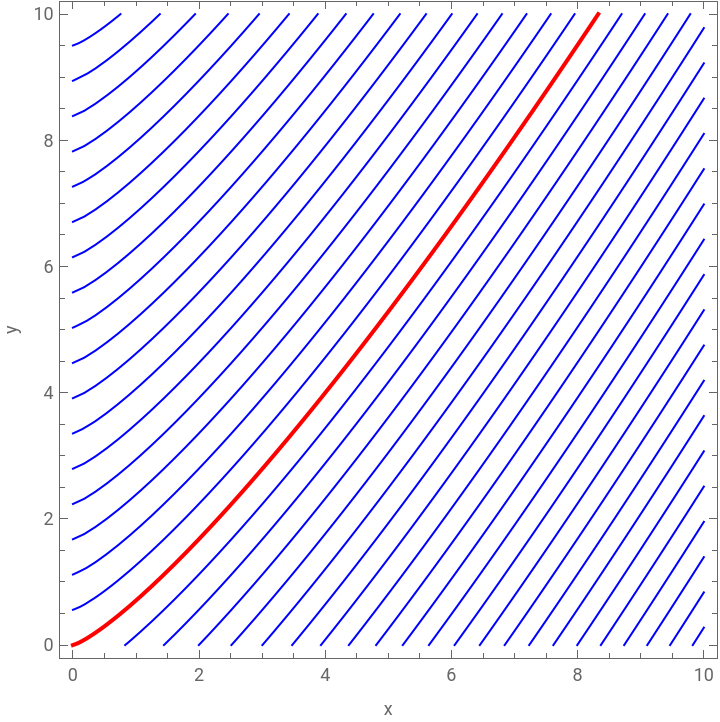
The evolution of the number of soldiers of armies and occurs along the hyperbola given by the equation The war evolves along that hyperbola, hence it depends on the starting point.
x
y
a-b==const.
2
x(t)
2
y(t)
The corresponding manifold of hyperbolas is separated by the line . If the starting point lies above this line, then the hyperbola finishes on the -axis. This means that in the course of the war army decreases to zero and army wins.
ax=by
y
x
y
Remark: Note that if the efficiency coefficients and are not constant then the equation determines a curve.
a
b
ax=by
Here is an interactive interface that illustrates the properties of the simplest model:
Out[]=




SDMon model
SDMon model
In this section we define the general model in a simple programmatic form using the paclet "MonadicSystemDynamics", [AAp2].
Remark: A better programmatic form would have equation elements that prevent (army) stocks to become negative.
Remark: Compared to the previous section, below we follow "wordier" but self-explanatory notation that helps model understanding, evaluation, and enhancements.
Here are the stocks:
In[]:=
aStocks=<|X[t]->"Soldiers of army X",Y[t]->"Soldiers of army Y"|>;
Here are the rates:
In[]:=
aRates=fireEfficiencyX"Efficiency of force X ",fireEfficiencyY"Efficiency of force Y",fireEfficiencyXonY"Efficiency of force X on Y",fireEfficiencyYonX"Efficiency of force Y on X",growthX"Growth rate of force X due to new recruits",growthY"Growth rate of force Y due to new recruits",diseaseX"Disease rate in force X",diseaseY"Disease rate in force Y",fireFriendlyX"Friendly fire rate in force X",fireFriendlyY"Friendly fire rate in force Y";
Here are rules that assign concrete values to the rates:
Initial conditions (number of soldiers):
Lanchester (or Lotka-Volterra) interactions:
Osipov interactions:
Equations:
Make the model data structure:
Display the model in tabular format:
Direct model simulation
Direct model simulation
Here we follow the equations setup and data in the article [JE1].
Remark: The data in [JE1] is later revisited and new computations were made with almost the same results. See [RS1].
Here replace the constant term of the first equation in the generalized model with the growth function growthIwoJimaX.
Here create the monadic pipeline, put the fire efficiency rates found in [JE1], simulate the for battles number of days, and plot the result:
Calibration
Calibration
In this section we show that using optimization methods -- calibration -- we can obtain the same efficiency rates as the ones theoretically computed in [JE1] using the same data.
Remark: This should bring some confidence in using SDMon; and since the calibration process is easy to specify, it should encourage SDMon's use for other SD models.
Consider the following calibration targets that are "time series" each derived via linear interpolation from two data points -- the start- and end values of the number of soldiers for each army:
Here is a model setup pipeline:
Here is a calibration pipeline that specifies:
1
.Target time series of the stocks
2
.Parameters to calibrate
3
.Parameter ranges, within which to search the calibration values
4
.Distance function from the computed time series to the target time series
5
.Parameters for NMinimize
Here we plot the simulated army sizes using the calibrated values:
Here we use a more "complicated" distance function that takes only the known points of the time series:
Remark: Note that with that new calibration distance function we get almost the same results as the theoretically computed efficiency rates in [JE1]:
In[]:=
<|fireEfficiencyX -> 0.0106, fireEfficiencyY -> 0.0544|>
Future plans
Future plans
Here are a few directions to extend this work into:
◼
Inclusion of different types of forces
◼
Simulation of "will to fight"
◼
Easy with NDSolve and, hence, with SDMon.
◼
Inclusion of weapon and ammunition production stocks and related supply rates
◼
For example, as in [AA2].
◼
Modeling the war impact on countries' economics and populations
◼
Modeling the role of propaganda
◼
Make interactive interfaces with knobs for the parameters
◼
With selectors of scenarios based on known battles.
References
References
Articles
Articles
[AA1] Anton Antonov, "A monad for Epidemiologic Compartmental Modeling Workflows", (2021), MathematicaForPrediction at WordPress.
[AS1] Andrei Shatyrko, Bedrik Puzha, Veronika Novotná, "Comparative Analysis and New Field of Application Lanchester’s Combat Models", (2018), Post-conference proceedings of selected papers extended version Conference MITAV-2018, Brno, Czech Republic, 2018. P.118-133. ISBN 978-80-7582-065-5.
[JE1] J.H. Engel, "A verification of Lanchester's law", (1953), Journal of the Operations Research Society of America, Vol. 2, No. 2. (May, 1954), pp. 163-171. (JSTOR link.)
[NM1] Nikolai V. Mityukov. Determining the casualties of wars through Lanchester models, (2009), Historical Psychology and Sociology of History.
[NM1ru] Н. В. МИТЮКОВ, ОПРЕДЕЛЕНИЕ ЖЕРТВ ВОЙН ЧЕРЕЗ ЛАНЧЕСТЕРСКИЕ МОДЕЛИ, Историческая психология и социология истории 2/2009 122–140.
[RS1] Robert W. Samz, ⎡Some Comments on Engel's "A Verification of Lanchester's Law"⎦, (1972), Operations Research, Vol. 20, No. 1 (Jan. - Feb., 1972), pp. 49-52 (4 pages) (JSTOR link.)
Books
Books
[VA1] Vladimir I. Arnold, Rigid and soft mathematical models, 2nd ed. (2008), Moscow Center of Continuous Mathematical Education.
In Russian: Владимир И. Арнольд, "«Жесткие» и «мягкие» математические модели", (2008), М.: МЦНМО, 2014, 32 с. ISBN 978-5-94057-427-9.
In Russian: Владимир И. Арнольд, "«Жесткие» и «мягкие» математические модели", (2008), М.: МЦНМО, 2014, 32 с. ISBN 978-5-94057-427-9.
Packages, paclets
Packages, paclets
[AAp1] Anton Antonov, EpidemiologicalModeling, WL paclet, (2023), Wolfram Language Paclet Repository.
Repositories
Repositories
CITE THIS NOTEBOOK
CITE THIS NOTEBOOK
Generalized Lanchester combat models
by Anton Antonov
Wolfram Community, STAFF PICKS, October 25, 2023
https://community.wolfram.com/groups/-/m/t/3055705
by Anton Antonov
Wolfram Community, STAFF PICKS, October 25, 2023
https://community.wolfram.com/groups/-/m/t/3055705