Neural networks can easily learn to regress cubic polynomials of type , but how do they do that? Results show that they internally access a variable , which is surprisingly close to the substitution used in the first step of the Cardano method for solving cubic polynomials.
y+a+x+b
3
x
2
x
tx+0.3a
tx+
a
3
Introduction
Introduction
MRI Scan of an NN
MRI Scan of an NN
What are the techniques used to interpret the behavior of an NN? Some might accept the cliché that NNs are black-box and we cannot really understand their inner workings. If you don’t accept this as absolute truth and you are willing to at least try to poke into the brain of an NN there are two main white-box interpretability techniques. The first technique relies on the analysis of individual neurons and answers the question “what’s the concept associated with a specific neuron?”. To answer this question, you can feed various inputs to your NN, measure the neurons’ activations and try to draw correlations such as “neuron #14 fires for and it is invariant to ”. Unfortunately, this often turns out to be an impossible task. Research has shown that neurons are polysemantic. Namely, the model reuses the same neuron for unrelated concepts. This happens because of the training pressure to compress a number of concepts that is inevitably greater than the number of neurons at disposal. In large language models, it was found that the same neuron fires both for “baseball” and “academic citations”. The clean 1-to-1 mapping between neurons and concepts that would make interpretability easy simply does not exist in most models. Similar noisy results were gathered in early efforts in trying to interpret the cubic polynomial regression NN.The second technique is to train a Sparse Autoencoder (SAE) on top of an activation layer of the NN to extract a more fine-grained representation of their concepts. From now on, I am gonna use the term feature, to indicate the NN-equivalent of human concepts. To understand what a SAE is, it is worth first explaining what a standard autoencoder is. A regular autoencoder is an MLP trained to compress and reconstruct an input vector. As an example, it might take a 100-dim vector as input, pass it through the encoder layer to compress it to a 50-dim vector and then feed it through the decoder to reconstruct the original 100-dim output vector. The encoder and the decoder are trained to minimize the reconstruction loss. Of course, the reconstruction cannot be fully accurate and some information is inevitably lost in the compression step.A SAE is like a standard autoencoder with the difference that it encodes the input vector into a larger dimension vector. If the training goal would simply be to minimize the reconstruction loss, the task would be trivial: the SAE would learn to use the identity matrix as encoder. But that wouldn’t tell us anything interesting. Therefore, we add a sparsity penalty to the training loss: the SAE is incentivized to encode the input vector into a sparse intermediate vector, namely a vector that can only have a limited number of non-zero elements.Going back to our context, we train a SAE on top of the last 15-dim activation layer of our NN. More concretely, we train (using an external python library) a 64-dim SAE with TopK=4. This means that it would be trained to learn 64 features and each encoded activation will be expressed in, at most, 4 features. To train the SAE, we sample 200k activations from the last activation layer of our NN for random input combinations . The learned parameters are (used for encoding) and (used for decoding). More specifically, given an activation vector , the sparse feature activation vector is defined as and the reconstructed activation vector is defined as zD. To assess the quality of a trained SAE, we measure the coefficient of the reconstruction on held-out activation vectors. The coefficient of the trained SAE is , indicating a close-to-lossless reconstruction.But why even bother training a SAE? It turns out that, while the activation vector is dense and difficult to interpret, the vector breaks down the polysemantic neurons into monosemantic components. This is possible thanks to the two key mechanisms that regulate the SAE: dimension expansion and sparsity. The expanded dimension provides enough space for every single feature to have its own dedicated “slot”. The sparsity requirement forces disentanglement.
b≤-2
a
(x,a,b)
Wandb
D
a
zReLU(Wa+b)
a
2
R
a
2
R
0.995
z
Out[]=
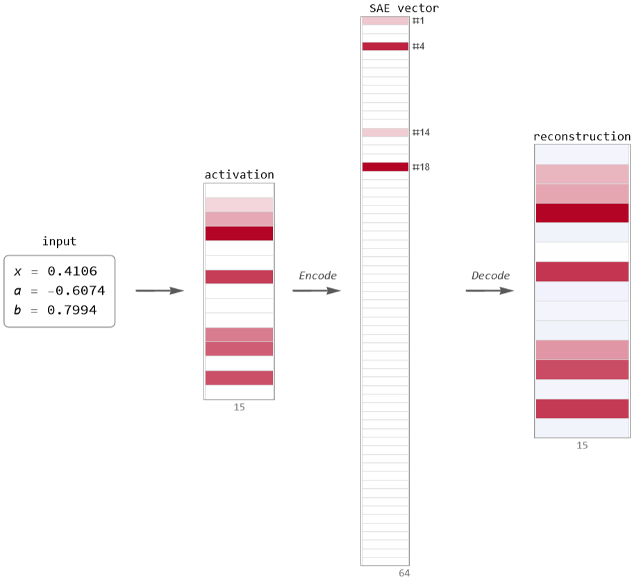
So, how can SAE help us understand what’s going on inside an NN? This is not so straight-forward.
The previous figure tells us that, for the given set of input, layer-4 activates four features: feature #1, #4, #14 and #18. And the second and fourth features are the ones that activate the most.
So this, by itself, doesn’t help us to understand how an NN thinks. The SAE does not provide any human-interpretable label to interpret a feature. In fact, the SAE is trained in a completely unsupervised fashion and there’s no training pressure that privileges interpretability. So, how do we make sense out of these features?
Let’s look at how features are interpreted in the context of LLMs. Assume that we have trained a SAE on top of the activations of layer. To understand what feature corresponding to the index represents, the practice is to simply look at the inputs that maximally activate that feature and give a gut reaction on their interpretability. For example, Anthropic trained SAEs on top of Claude Sonnet and found a feature that activates on contexts (text or images) related to the Golden Gate Bridge. Much progress has been made since then and now we have complete SAE mapping of LLMs such as Gemma-4 and plausible labels for each of these features.
The gist is that, in order to understand the meaning of a feature, it is necessary to identify the least common denominator across all the scenarios in which that specific feature fires. So the first step is to come up with a hypothetical scenario in which we expect a certain feature to fire.
Based on the way we humans interpolate cubic polynomials, I made the hypothesis that the NN would recognize landmark points of a polynomial such as roots, critical points (roots of the derivative) and inflection point (where the concavity of the curve changes, or root of the second order derivative).
To understand whether an NN recognizes landmark points, I draw, for a polynomial parametrized by, the activation pattern over for all the 64 features. I also draw vertical dotted lines in proximity of the landmark points: in particular, red indicates the roots, blue indicates the critical points and green the inflection point. The figure shows, for the polynomial parametrized by and , the activation pattern of the 64 features and, right below, the actual shape of the polynomial.
The previous figure tells us that, for the given set of input
(x0.4106,a-0.6074,b0.7994)
So this, by itself, doesn’t help us to understand how an NN thinks. The SAE does not provide any human-interpretable label to interpret a feature. In fact, the SAE is trained in a completely unsupervised fashion and there’s no training pressure that privileges interpretability. So, how do we make sense out of these features?
Let’s look at how features are interpreted in the context of LLMs. Assume that we have trained a SAE on top of the activations of layer
ℓ
i
The gist is that, in order to understand the meaning of a feature, it is necessary to identify the least common denominator across all the scenarios in which that specific feature fires. So the first step is to come up with a hypothetical scenario in which we expect a certain feature to fire.
Based on the way we humans interpolate cubic polynomials, I made the hypothesis that the NN would recognize landmark points of a polynomial such as roots, critical points (roots of the derivative) and inflection point (where the concavity of the curve changes, or root of the second order derivative).
To understand whether an NN recognizes landmark points, I draw, for a polynomial parametrized by
(a,b)
x∈[-3,3]
a3
b-1
Out[]=
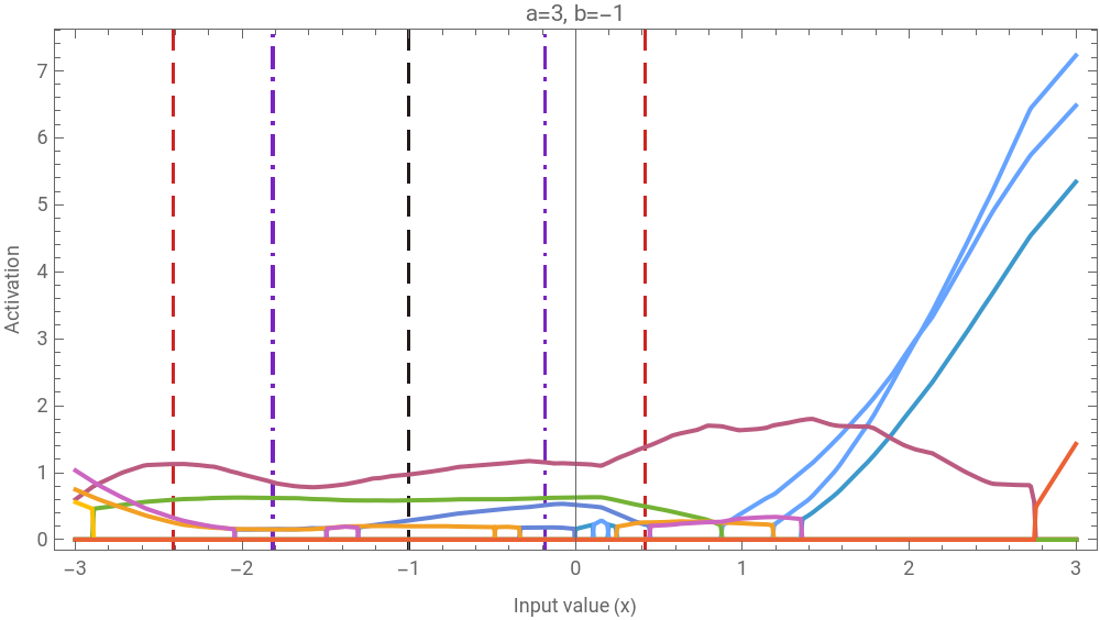


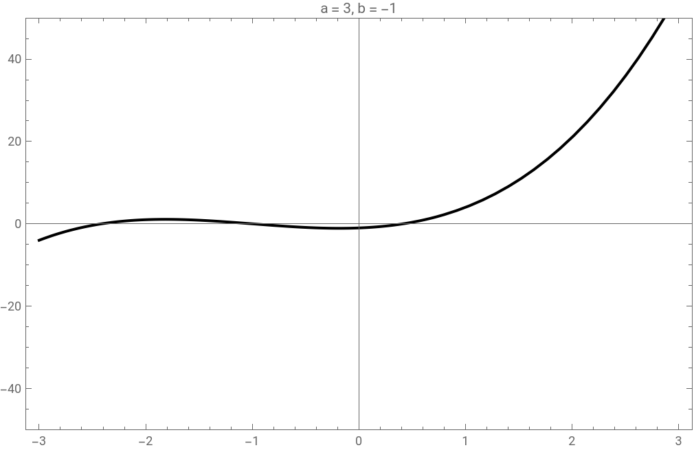
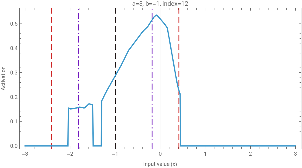
The picture is pretty complicated to understand. We can try to make it easier by isolating the activation patterns of individual features such as feature #12 or #18.
Out[]=
Out[]=
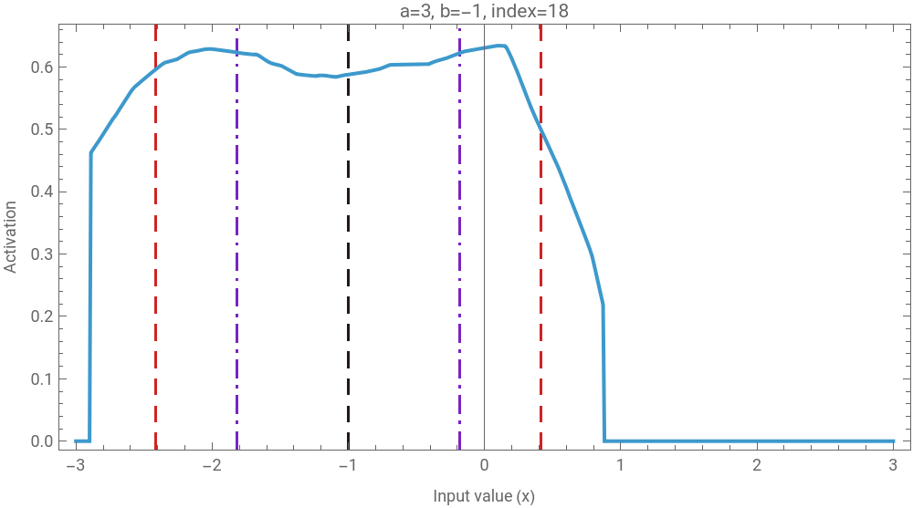
Looking at the activation pattern of feature #12 I see somewhat a pattern of bumps in proximity to critical points, and a fall in proximity of the second root. Let’s analyze the activation pattern of the same feature for a different polynomial.
Out[]=
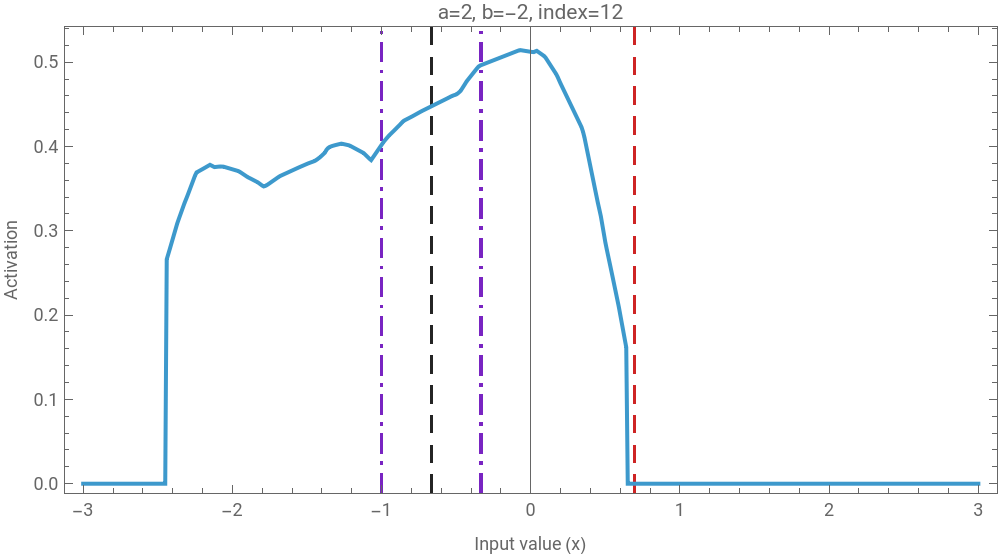
Let’s try to find out other “interesting” features. What are the features that have the highest correlation with the roots?
The “Aha!” Moment
The “Aha!” Moment
Why is a/3 Special? The Cardano Method
Why is a/3 Special? The Cardano Method
How Is the Feature Used? Manipulating the Brain
How Is the Feature Used? Manipulating the Brain
To measure the impact of the feature clamping, the forward pass is run on a model in which the real activation is replaced by the activation derived after manipulation.
A good example of model manipulation comes from Anthropic. The researchers identified, via SAE, a specific feature in Sonnet that looks like firing in context related to the Golden Gate Bridge. In order to verify their interpretation they tuned the activation of that feature artificially high and observed the behavior of the model. The model started mentioning the Golden Gate Bridge in every response, demonstrating that the feature was labelled correctly.
It seems like the diagonal band features are somewhat associated with a multiplicative effect or vertical stretch of the curve and the magnitude of the transformation is proportional to the multiplicative factor applied to manipulate such features.
We notice that the error is not a consequence of the feature manipulation but it is attributable to the “standard” SAE reconstruction error. You can see that, where the multiplicative factor is 1 (no manipulation was applied), the error is still present.
One further experiment that I plan to run is to train a SAE on top of the middle layers of the NN, which are often associated with abstract thinking.
How Do Abstractions Emerge?
How Do Abstractions Emerge?
“If I had more time, I would have written a shorter letter”
— Blaise Pascal
— Blaise Pascal
Acknowledgements
Acknowledgements
I want to thank Christian Pasquel and my group-mates Caden Lafollette, Mohamed AlBegaowe and Ahmet Erhan AVCI, for their decisive and continuous support during the project.
Thanks to Júlia Campolim for helping me debugging my code.
Thanks to Nora Popescu for letting me use her M5 processor.
Thanks to Brian Mboya for review and feedback.
Finally, special thanks to Stephen Wolfram. His foundational questions about the nature of abstractions will keep me busy for years.
Thanks to Júlia Campolim for helping me debugging my code.
Thanks to Nora Popescu for letting me use her M5 processor.
Thanks to Brian Mboya for review and feedback.
Finally, special thanks to Stephen Wolfram. His foundational questions about the nature of abstractions will keep me busy for years.
AI Disclosure
AI Disclosure
The following generative AI tools were used in this project: Claude Fable 5, Claude Sonnet 5, Google Gemini 3.1 Pro. The former two were used to generate code for illustrations, for proof-reading and to find “interesting” activation patterns, while the latter was used for brainstorming. All code and written content was reviewed, understood and approved by the author.
CITE THIS NOTEBOOK
CITE THIS NOTEBOOK
Interpreting How Neural Nets Regress Cubic Polynomials
by Enrico Bottazzi
Wolfram Community, STAFF PICKS, July 16, 2026
https://community.wolfram.com/groups/-/m/t/3763526
by Enrico Bottazzi
Wolfram Community, STAFF PICKS, July 16, 2026
https://community.wolfram.com/groups/-/m/t/3763526