Wolfram Cloud Document

Abstract. We present a concise, reproducible Wolfram Language workflow for modeling and visualizing the planar dynamics of an undamped double pendulum. Motivated by the need for a clear, teachable example of nonlinear multi-body motion, we derive the equations via the Lagrangian approach from the generalized coordinates

θ

1

and

θ

2

, then solve them numerically over a chosen time window. Time series, a

θ

2

-

θ

1

phase portrait, and

(x,y)

path traces are generated by the notebook, and strong energy exchange and tangled, non-closing trajectories indicative of chaos are revealed. The workflow is intended for students and instructors seeking an extensible template to begin studying chaotic dynamics.

1. System Setup and Kinematics

A double pendulum is formed by suspending one pendulum from the end of another. Although the setup is mechanically simple, it provides a striking example of a system that can exhibit chaotic motion. Consider a double pendulum consisting of two equal point masses

m

1

=

m

2

=0.25

kg, connected by rigid, massless wires of lengths

l

1

=0.22

m and

l

2

=0.18

m. The angles that the two wires make with the vertical are denoted by

θ

1

and

θ

2

, as shown in Fig. 1. The gravitational acceleration is taken to be

g=9.81m/

2

s

.

Define the system parameters by specifying the masses, pendulum lengths, and gravitational acceleration:

In[]:=

m1=m2=0.25;l1=0.22;l2=0.18;g=9.81;

Determine the location of the fixed pivot point and the instantaneous positions of the pendulum masses:

In[]:=

o={0,0,0};p1={1,-2,0};p2={2.5,-3,0};

Create labeled elements and pendulum geometry:

In[]:=

labeledGrphics=Style[Inset[#1,#2],16,Italic,FontFamily->"Times",Bold]&@@@

Labels

,

Shapes

;

Render a Graphics3D of the double pendulum system (not to scale):

In[]:=

PaneGraphics3DlabeledGrphics,

Options

,ImageSize->Scaled[1]

Out[]=

The instantaneous coordinates of the two masses,

(

x

1

(t),

y

1

(t))

and

(

x

2

(t),

y

2

(t))

, can be expressed in terms of the lengths

l

1

and

l

2

, together with the time-dependent angles

θ

1

(t)

and

θ

2

(t)

, as follows:

x

1

(t)=

l

1

sin(

θ

1

(t))

y

1

(t)=-

l

1

cos(

θ

1

(t))

x

2

(t)=

l

1

sin(

θ

1

(t))+

l

2

sin(

θ

2

(t))

y

2

(t)=-

l

1

cos(

θ

1

(t))-

l

2

cos(

θ

2

(t))

(1)

Express the instantaneous coordinates of the masses in terms of the lengths and time-dependent angles:

In[]:=

x1[t_]:=l1Sin[θ1[t]]y1[t_]:=-l1Cos[θ1[t]]x2[t_]:=l1Sin[θ1[t]]+l2Sin[θ2[t]]y2[t_]:=-l1Cos[θ1[t]]-l2Cos[θ2[t]]

The kinetic energy

(t)

accounts for the motion of both pendulum masses through their speeds

v

1

(t)

and

v

2

(t)

, while the potential energy

(t)

represents their gravitational energy based on vertical distances

y

1

(t)

and

y

2

(t)

:

(t)=

1

2

m

1

2

v

1

(t)+

1

2

m

2

v

2

(t)

(t)=

m

1

g

y

1

(t)+

m

2

g

y

2

(t)

(2)

The speeds can be defined in terms of the time derivatives of the coordinates, with the dot notation indicating differentiation with respect to time:

v

1

(t)=

2



x

1

(t)+

2



y

1

(t)

v

2

(t)=

2



x

2

(t)+

2



y

2

(t)

(3)

Formulate the kinetic and potential energy of the system (derivatives appear as dashes in the code):

In[]:=

[t_]:=

1

2

m1(

2

x1'[t]

+

2

y1'[t]

)+

1

2

m2(

2

x2'[t]

+

2

y2'[t]

);[t]//Simplify

Out[]=

0.0121

2

′

θ1

[t]

+0.0099Cos[θ1[t]-θ2[t]]

′

θ1

[t]

′

θ2

[t]+0.00405

2

′

θ2

[t]

In[]:=

[t_]:=m1gy1[t]+m2gy2[t];[t]//Simplify

Out[]=

-1.0791Cos[θ1[t]]-0.44145Cos[θ2[t]]

2. Lagrangian and Equations of Motion

In relatively complex dynamical systems, the Lagrangian formalism is often preferred because it works with scalars (kinetic and potential energies) rather than vectors (forces and accelerations as in Newton’s laws). This avoids splitting forces into components, which makes the analysis much simpler for systems like the double pendulum. The Lagrangian of a mechanical system is defined as the difference between its kinetic and potential energies:

ℒ(t)=(t)–(t)

. A discussion of the double pendulum using Newtonian mechanics can be found in the double pendulum topic of the Wolfram documentation.

Define the Lagrangian of the system:

In[]:=

ℒ[t_]:=[t]-[t];ℒ[t]//Simplify

Out[]=

1.0791Cos[θ1[t]]+0.44145Cos[θ2[t]]+0.0121

2

′

θ1

[t]

+0.0099Cos[θ1[t]-θ2[t]]

′

θ1

[t]

′

θ2

[t]+0.00405

2

′

θ2

[t]

To derive the equations of motion for the double pendulum, we apply the Euler–Lagrange equation to the generalized coordinates

θ

1

and

θ

2

. For each angle, the equation takes the form:

d

dt

∂ℒ

∂



θ

1

-

∂ℒ

∂

θ

1

=0

d

dt

∂ℒ

∂



θ

2

-

∂ℒ

∂

θ

2

=0

(4)

Derive the equations of motion using the Euler–Lagrange equations:

In[]:=

diffEqns=Simplify[D[D[ℒ[t],D[#,t]],t]-D[ℒ[t],#]]==0&/@{θ1[t],θ2[t]}

Out[]=

{1.0791Sin[θ1[t]]+0.0099Sin[θ1[t]-θ2[t]]

2

′

θ2

[t]

+0.0242

′′

θ1

[t]+0.0099Cos[θ1[t]-θ2[t]]

′′

θ2

[t]0,0.44145Sin[θ2[t]]-0.0099Sin[θ1[t]-θ2[t]]

2

′

θ1

[t]

+0.0099Cos[θ1[t]-θ2[t]]

′′

θ1

[t]+0.0081

′′

θ2

[t]0}

Or, use the built-in EulerEquations function to obtain the same result:

In[]:=

Needs["VariationalMethods`"]EulerEquations[ℒ[t],{θ1[t],θ2[t]},t]

Out[]=

{-1.0791Sin[θ1[t]]-0.0099Sin[θ1[t]-θ2[t]]

2

′

θ2

[t]

-0.0242

′′

θ1

[t]-0.0099Cos[θ1[t]-θ2[t]]

′′

θ2

[t]0,-0.44145Sin[θ2[t]]+0.0099Sin[θ1[t]-θ2[t]]

2

′

θ1

[t]

-0.0099Cos[θ1[t]-θ2[t]]

′′

θ1

[t]-0.0081

′′

θ2

[t]0}

Alternatively, use the resource function EulerEquations to obtain the same result:

ResourceFunction["EulerEquations"][ℒ[t],{θ1[t],θ2[t]},t]

Out[]=

{-1.0791Sin[θ1[t]]-0.0099Sin[θ1[t]-θ2[t]]

2

′

θ2

[t]

-0.0242

′′

θ1

[t]-0.0099Cos[θ1[t]-θ2[t]]

′′

θ2

[t]0,-0.44145Sin[θ2[t]]+0.0099Sin[θ1[t]-θ2[t]]

2

′

θ1

[t]

-0.0099Cos[θ1[t]-θ2[t]]

′′

θ1

[t]-0.0081

′′

θ2

[t]0}

We then set the initial conditions (

θ

1

(0)=π/2,



θ

1

(0)=0,

θ

2

(0)=π/2,

and



θ

2

(0)=0

), combine the equations of motion with these conditions into a single initial-value problem, and solve it numerically.

Set the initial conditions for both pendulum angles and their velocities:

In[]:=

initCond={θ1[0]==π/2,θ1'[0]==0,θ2[0]==π/2,θ2'[0]==0};

Combine the differential equations with the initial conditions into a single system:

In[]:=

eqnsSet=Join[diffEqns,initCond];eqnsSet//Column

Out[]=

1.0791Sin[θ1[t]]+0.0099Sin[θ1[t]-θ2[t]]

2

′

θ2

[t]

+0.0242

′′

θ1

[t]+0.0099Cos[θ1[t]-θ2[t]]

′′

θ2

[t]0

0.44145Sin[θ2[t]]-0.0099Sin[θ1[t]-θ2[t]]

2

′

θ1

[t]

+0.0099Cos[θ1[t]-θ2[t]]

′′

θ1

[t]+0.0081

′′

θ2

[t]0

θ1[0]

π

2

′

θ1

[0]0

θ2[0]

π

2

′

θ2

[0]0

Solve the system numerically over the chosen time interval:

In[]:=

sol=First[NDSolve[eqnsSet,{θ1,θ2},{t,0,15}]]

θ1InterpolatingFunction

Domain: {{0.,15.}}

Output: scalar

,θ2InterpolatingFunction

Domain: {{0.,15.}}

Output: scalar



3. Results and Visual Analysis

Fig. 2 shows two complementary views over 0–15 s. Fig. 2a plots the time series of

θ

1

(t)

and

θ

2

(t)

, and Fig. 2b shows the angle–angle trajectory

θ

2

(t)

versus

θ

1

(t)

. In Fig. 2a,

θ

2

(t)

displays larger excursions and intermittent bursts of rapid growth, consistent with strong energy exchange and sensitivity to initial conditions. In contrast,

θ

1

(t)

remains more bounded with smaller-amplitude oscillations. In Fig. 2(b), the trajectory traces a tangled, non-closing path, indicating aperiodic motion and chaos.

Plot the time series of θ₁(t), θ₂(t) and the angle–angle trajectory (θ₂ vs. θ₁):

RowPlotEvaluate[#],{t,0,15},

Options

,ParametricPlot#,{t,0,15},

Options

," "&[{θ1[t],θ2[t]}/.sol]

Out[]=

	θ₁(t)
	θ₂(t)

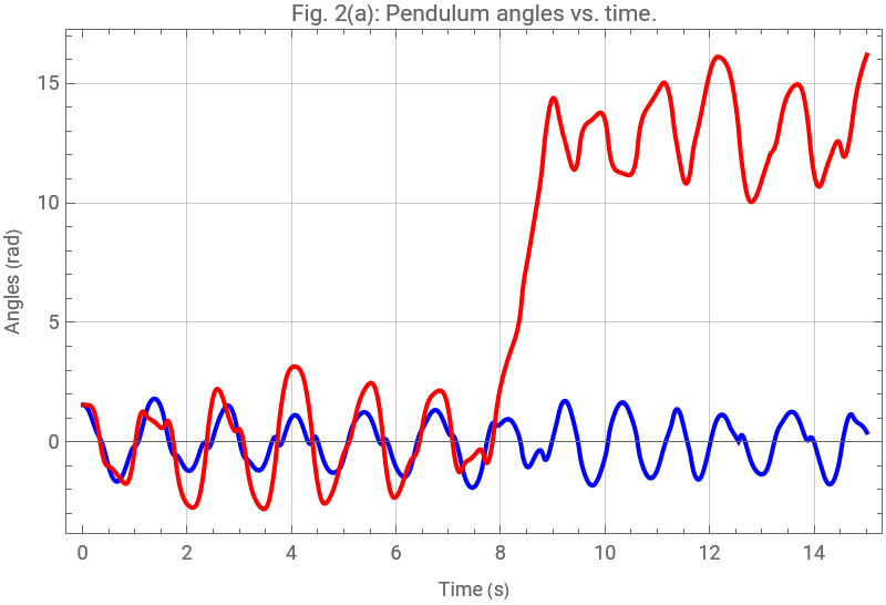
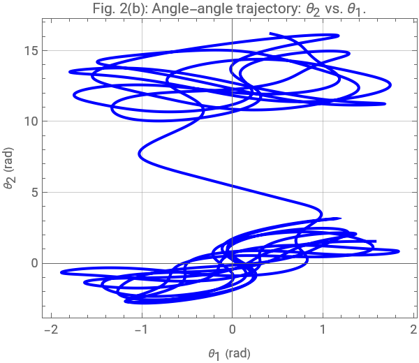
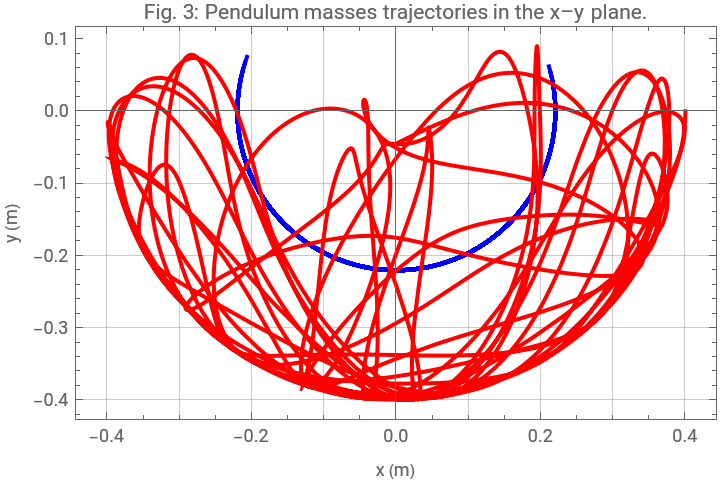
Fig. 3 plots the

x–y

trajectories of the two pendulum masses over 0–15 s. Imagine each mass carrying a pen that draws its path as it moves—

m

1

in blue and

m

2

in red. The inner, shorter track belongs to

m

1

, which stays closer to the pivot, while

m

2

sweeps a wider region, marked by loops and cusps that indicate rapid direction changes. The dense self-intersections and absence of a closed loop indicate aperiodic motion and ongoing energy exchange between the arms.

Plot the

x–y

trajectories of the two pendulum masses: