Geographic Distortions
George Varnavides, 01/29/2021
George Varnavides, 01/29/2021
◼
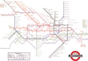
I’ve long been fascinated with transportation maps, and in particular the revolutionary re-design of the london-underground map by Harry Beck in 1933.
◼
In his iconic design, which has since been adopted by most transportation maps, Harry Beck deliberately sacrifices geographic accuracy for visual clarity of information - by using equally-spaced stations on straight lines with only 45/90 degree bends
◼
Here, we show how the local coordinate system is distorted through the years as more stations get added to display the information clearly
◼
A note on the old transportation map figures:
◼
I’ve had these on my machine from an old visual information project
◼
I don’t believe these are publicly available on the web, so I’ll refrain from attaching these on the post
◼
Contact me if you’re interested, and I can point you to where I got them from
◼
References:
◼
Beineke D. Verfahren zur Genauigkeitsanalyse fur Altkarten. Munchen: Universitat der Bundeswehr; 2001.
◼
Jenny, Bernhard, and Lorenz Hurni. “Studying cartographic heritage: Analysis and visualization of geometric distortions.” Computers & Graphics 35.2 (2011): 402-411.
London Underground Maps
London Underground Maps
◼
First, we start by importing a number of these old transportation maps
In[]:=
SetDirectory[NotebookDirectory[]];londonUndergroundMapFiles=FileNames["london_underground_map_*.png","maps"];years=ToExpression[StringSplit[#,{"_","."}][[-2]]]&/@londonUndergroundMapFilesDo[distortedMap[year]=Import[StringTemplate["maps/london_underground_map_`1`.png"][year]],{year,years}]
Out[]=
{1933,1938,1940,1944,1945,1946,1948,1949,1951,1958,1960,1964,1968,1970,1972,1973,1977,1985,1987,1990,1994,1999,2009,2011,2016,2020}
◼
The original Harry Beck 1933 map
In[]:=
Rasterize[distortedMap[1933],RasterSize600]
Out[]=
◼
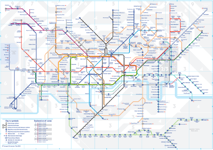
The current (May 2020) London underground map
◼
While a great many new stops have been added, the map is still faithful to the original style
In[]:=
Rasterize[distortedMap[2020],RasterSize600]
Out[]=
◼
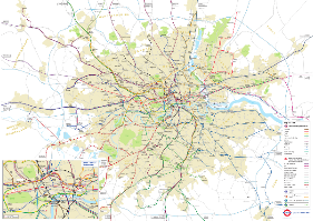
This can be compared to a geographically-accurate map of the London Underground (from 2014)
In[]:=
geographicallyAccurateMap[2014]=Import["maps/geographically_accurate_map_2014.png"];Rasterize[geographicallyAccurateMap[2014],RasterSize600]
Out[]=
Reference Points
Reference Points
◼
In order to compare the transportation maps to the geographically accurate one, we require a set of reference points in the respective coordinate systems
◼
The obvious choice is to use the stations available at that point in time
In[]:=
referencePointFiles=FileNames["image_dims_reference_points_*.txt","reference_points"];referenceYears=ToExpression[StringSplit[#,{"_","."}][[-2]]]&/@referencePointFilesDo[referencePoints[year]=Import[StringTemplate["reference_points/image_dims_reference_points_`1`.txt"][year],"Data"],{year,referenceYears}]
Out[]=
{1933,1938,1940,1945,1946,1948}
◼
These were tediously collected in image dimension units, using `Get Coordinates`
◼
I tried automating this briefly using Image Processing, but couldn’t get satisfactory results
◼
Any advice on this would be greatly appreciated!
Global Transformations
Global Transformations
◼
First, the maps have different coordinate systems (and often image dimensions/aspect ratios)
◼
So we find the best global transformation to align the ‘geographically accurate’ locations to the transportation map’s coordinate system
In[]:=
undergroundMapPoints[year_]:=referencePoints[year][[All,2;;3]]geographicallyAccuratePoints[year_]:=referencePoints[year][[All,4;;5]]
In[]:=
globalTransformation[year_]:=Block[{error,tf},{error,tf}=FindGeometricTransform[undergroundMapPoints[year],geographicallyAccuratePoints[year],Method"Linear",TransformationClass"Similarity"];tf]
◼
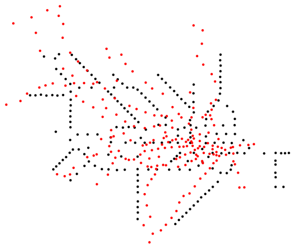
Superimposing the two we get
In[]:=
{undergroundMapPoints[1933]//Point,Red,globalTransformation[1933][geographicallyAccuratePoints[1933]]//Point}//Graphics
Out[]=
Displacement Vectors
Displacement Vectors
◼
A simple way of visualizing the distortion, is simply to associate each reference point to where it would like had the map been ‘as accurate’ as the geographically accurate locations
◼
Meaning we’ll draw displacement vectors from the transportation map stations to the respective locations following our global transformation
Distortion Grids
Distortion Grids
◼
To go further, we wish to setup a local grid and see how it transforms to accommodate the displacement vectors
◼
We start with a regularly spaced grid spanning the geographically accurate map’s coordinate system
◼
and distort it (rotate, scale, translate) according to the global transformation above
◼
A (hacky) way of joining nearest points to display a grid
◼
We can the use a multi-quadratic interpolation to extract the local grid displacements to match the displacement vectors
◼
where U, V are vectors of horizontal and vertical displacement vectors respectively,
◼
and a,b are the vectors of local transformation parameters we’re trying to fit
◼
The distorted grid’s displacement vectors are then given by the weighted sum:
◼
Putting everything together to construct our displacement grid:
◼
And overlay the distortion grid on our transportation map
◼
And a look at the first six London underground distorted grid maps