WOLFRAM NOTEBOOK

Perception & Analysis Pt II

By David Ameneyro. April 17, 2020.
In the last post we looked at how different encodings of the same data affect our human ability to process that data. When viewed in an ArrayPlot with 1s being black squares and 0s being white squares, we could easily discern between data produced by different cellular automata as our visual system detected different textures for different programs. We could not discern differences when encoded as actual 1s and 0s or when converting those 1s and 0s to Base 10 integers.​
​In this post we’ll assess how effective different programmatic approaches are at handling different encodings. That is, can Mathematica’s built-in machine learning functions reliably distinguish between two different cellular automata outputs.

Classifier Function

The Wolfram Language has a built-in function—Classify—which will take a tagged data set, evaluate different modeling methods, and use the best one to train a Classifier function to classify new data into the specified classes.
This function works on many different types of data so we can use it to evaluate all three of the encodings we used above (array plots , base 2 arrays, and base 10 arrays).

Array Plots

For the first test we’ll use array plots.
Step 1: Generate and label training data
The command below renders and labels 50 random examples from each possible CA rule. Using Parallelize enables multiple kernels to evaluate the command in parallel. The basic home license allows eight simultaneous kernels, however, my 7 year old MacBook only has two cores so I can only use two at a time. The decrease in time is still considerable at 60% better than without using a Parallelize.
In[]:=
allarrayplotrulestrain=Parallelize[Table[Thread[Table[ArrayPlot[CellularAutomaton[n,RandomInteger[1,100],{50,{-50,50}}]],50]Table[StringJoin["Rule",ToString[n]],50]],{n,255}]]//Flatten;
Step 2: Train Classifier
The command below is simple, requiring only the Classify function with one argument, the training data. You will notice that I specify the Method the classifier uses. This is only because I already ran the classifier once and it chose Logistic Regression as the best method. I lost that model when my computer quit, so I specified it here to save time. See footnote 1 for more information on the model
In[]:=
arrayplotruleclassifier=Classify[allarrayplotrulestrain,Method"LogisticRegression"]
CloudPut[arrayplotruleclassifier,"arrayplotruleclassifier"]
In[]:=
cloudarrayplotruleclassifier=CloudGet["arrayplotruleclassifier"]
Out[]=
ClassifierFunction
Input type: Image
Number of classes:
255
Unable to save data.
Step 3: Generate and label test data
This is the same procedure as Step 1
In[]:=
allarrayplotrulestest=Parallelize[Table[Thread[Table[ArrayPlot[CellularAutomaton[n,RandomInteger[1,100],{50,{-50,50}}]],50]Table[StringJoin["Rule",ToString[n]],50]],{n,255}]]//Flatten;
Step 4: Test the Classifier
This step runs the trained classifier on the test data from Step 3, and then provides two different evaluations, and accuracy percentage and a Confusion Matrix.
In[]:=
arrayplotclassifierresults=ClassifierMeasurements[cloudarrayplotruleclassifier,allarrayplotrulestest]
Out[]=
ClassifierMeasurementsObject
Classifier: LogisticRegression
Number of test examples: 12750
Unable to save data.
In[]:=
arrayplotclassifierresults/@{"Accuracy","ConfusionMatrixPlot"}//TableForm
Out[]//TableForm=
0.714902
Conclusion
Accuracy
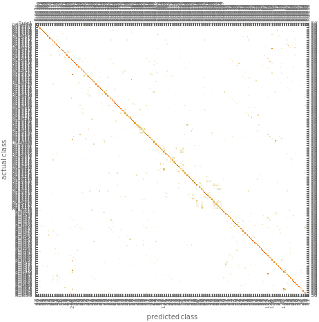
The Classifier had 71% accuracy at distinguishing between different cellular automata outputs. It’s hard to evaluate this performance against our human performance in the last post since we are running two different tests. We just tested whether we could identify where one pattern ends and another begins, while this test had the computer identify each individual CA, some of which have very similar looking outputs which I doubt I could distinguish between side by side (example below). The 72% accuracy will be better when we can compare against the other methods below.
Confusion Matrix
The confusion matrix is more of a visual assessment than an actual objective measure. One axis is the actual class and the other is the predicted class. Perfect accuracy would be a diagonal line from top left to bottom right. In this we see a strong diagonal line with some misses scattered throughout. Again, this will be a more useful tool when we compare to the other methods below.

1s and 0s

This next evaluation will be the same as the above, except that we will not plot the arrays as black and white squares but will instead keep them as lists of 1s and 0s.
Note that since the steps are the same as above, I will not break up into separate sections. I’ve hidden most of the steps to make it cleaner and am only showing the final steps. You can open the code input cell to examine/run the steps by double-clicking the cell grouping line along the right side of the notebook.
In[]:=
all1s0srulestrain=Parallelize[Table[Thread[Table[CellularAutomaton[n,RandomInteger[1,100],{50,{-50,50}}],50]Table[StringJoin["Rule",ToString[n]],50]],{n,255}]]//Flatten;
In[]:=
classifierresults1s0s/@{"Accuracy","ConfusionMatrixPlot"}//TableForm
Out[]//TableForm=
0.0627451
Conclusion
These results shocked me. The data was encoded in 1s and 0s, the language of computers, and the function only achieved a 6% accuracy. This is also evident in confusion matrix where we can see only a faint diagonal line but mostly random results. Completely random results would achieve 0.4% accuracy so the classifier did improve above random.

Base 10

Same evaluation as the first two. These cells are also closed except for the results.
In[]:=
allbase10rulestrain=Parallelize[Table[Thread[Table[FromDigits[#,2]&/@CellularAutomaton[n,RandomInteger[1,100],{50,{-50,50}}],50]Table[StringJoin["Rule",ToString[n]],50]],{n,255}]]//Flatten;
In[]:=
base10classifierresults/@{"Accuracy","ConfusionMatrixPlot"}//TableForm
Out[]//TableForm=
0.0908235
Conclusion
With 9% accuracy the classifier performed better on this encoding than in 1s and 0s, but in the end even the computer did better on visual data.
I suspect that since these machine learning functions are pre-trained with whatever data Wolfram Research assumes its userbase will use most often, they may be biased to performing better on image data simply because the company thought users would use these automated functions for images or other non-traditional data and use classic statistical analysis on integer data. However, that conclusion is highly speculative, and not based on any evidence.
With more time and compute power, we could train a neural net from scratch on each encoding and see how they perform from there.

Cluster Analysis

Mathematica has several built-in cluster analysis functions which can take many different forms of data and group them together based on similarities. We’ll perform the same basic workflow as above by feeding the three different encodings of data into the same function to see how they perform.

Nearest Neighbors

This function finds and graphs nearest neighbors automatically. The function didn’t work well until I specified how many neighbors to connect each vertex to, so you can see that i chose to specify 3 nearest neighbors. While we were originally testing whether the computer could make effective distinctions between CA outputs, we can assume that if they’re clustered based on similarities, that is effectively equivalent to not clustering differentiated data.
Note that the NearestNeighborGraph function had difficulty with the base 2 data. I had to significantly pare down that data by limiting it to 50 randomly chosen CAs with only 20 steps for each, compared to all 255 rules with 50 steps each which we’ve been using for all other analyses.
The resulting graphs are difficult to evaluate objectively since they don’t have numeric values for cluster effectiveness, and also difficult to evaluate subjectively since the graphs themselves don’t highlight clusters. The Wolfram language does have further built-in commands for finding clusters within graphs and highlighting them. We’ll use those commands here:
Conclusion
These functions made it easier to distinguish between clusters. The graphs have 10, 5, and 8 clusters respectively. Since the data isn’t effectively labeled it’s hard to even see a representative rule for each of the clusters, or whether I agree with the way the CAs have been clustered. Note: if you know how I can modify the code to get better labeling, please let me know!
That said, by separating the commands above, and just using the FindGraphCommunities function on the array plots graph, I can see that the original Nearest Neighbors function did not cluster the rules in a way that made sense to me. There are many visually similar CAs that were in separate clusters, so I am unsure on what basis those array plots were evaluated.
You can see that command here, though I won’t show the output since it is very long.

Clustering Components

This function also finds clusters within data, but instead of graphing that data it allows us to highlight those clusters by using it in conjunction with the Colorize function.
For this analysis we will generate two different CA arrays and join them together in a single array (similar to how we did in the last post), and see if the function can pick out key components such as triangles or other structures.
I’ve chosen a few CAs that have highly differentiated array plots but that are still representative of many CAs.
Conclusion
The function was unable to find any real clusters in any of the images. The results show that the function indicated black squares as one cluster and white squares as the other, which does not give us any more information about the array plots than we already had and does not helps us differentiate between them. Note that since none of the array plots showed interesting results I am only showing three random plots.

Feature Space Plot

FeatureSpacePlot is just a mashup of the DimensionReduce and ListPlot functions. DimensionReduce functions exactly as the name describes and reduces multi-dimensional objects in the specified number of dimensions (in this case {x, y}) using
Conclusion
Like the Nearest Neighbor Graphs above, these can’t be judged objectively. Subjectively, the function did a decent job with the array plots, separating different looking CAs. The base 2 data looks essentially random, and the Base 10 data looks somewhere between the base 2 and the array plots. Unfortunately, I didn’t readily find a function for highlighting the clusters in the plot like we used for the Nearest Neighbor Graphs. If you know of a better way to evaluate these, let me know!

Criticisms

Limiting Classes

Different cellular automata can produce similar outputs, and we could have grouped the CAs together based on these similarities (e.g. CAs that produce triangles vs diagonal lines vs all black). These groupings would simplify the number of classes that our classifiers/cluster analyses had to learn, rather than making them work on a 255-class data set. It’s possible that with this simpler data, better accuracy could be achieved. It would also level the playing field between our human based tests in the first post and the computer analyses here.
See the footnote 2 for more on classes of CAs.

Next Time

There are a lot more built-in machine learning functions that we haven’t gotten to yet. I’d like to keep using these on cellular automata to see what we find. Additionally, we haven’t yet tried to crack these using traditional statistical techniques.

Did you like this post? Any ideas on other approaches I could have taken or ways to make my code more elegant? I'd love to hear from you!

Hit me up on Twitter (@ahmeneeroe) or email (david.ameneyro@gmail.com)

Footnotes

1. The Information function shows a lot of fun data on the model’s training and performance. See below for more info:
Wolfram Cloud

You are using a browser not supported by the Wolfram Cloud

Supported browsers include recent versions of Chrome, Edge, Firefox and Safari.


I understand and wish to continue anyway »

You are using a browser not supported by the Wolfram Cloud. Supported browsers include recent versions of Chrome, Edge, Firefox and Safari.