ABSTRACT (original article): Dirac notation is widely used in quantum physics and quantum programming languages to define, compute and reason about quantum states. This paper considers Dirac notation from the perspective of automated reasoning. We prove two main results: first, the first-order theory of Dirac notation is decidable, by a reduction to the theory of real closed fields and Tarski’s theorem. Then, we prove that validity of equations can be decided efficiently, using term-rewriting techniques. We implement our equivalence checking algorithm in Mathematica, and showcase its efficiency across more than 100 examples from the literature. CITATION (original article): Xu, Y., Barthe, G., & Zhou, L. (2025). Automating Equational Proofs in Dirac Notation. Proceedings of the ACM on Programming Languages, 9(POPL), 1227–1259. https://doi.org/10.1145/3704878
Find the package files here: https://zenodo.org/records/13995586
In[]:=
AppendTo[$Path, FileNameJoin[{NotebookDirectory[], "DiracDec"}]];Get["DiracAll`"]
Motivating Example
It is an interesting quantum information fact expressed as an equation of Dirac notation. Let’s see how DiracDec help to prove it.
The Problem Setting
The Problem Setting

The DiracDec Encoding
The DiracDec Encoding
In[]:=
DiracCtx={M->OType[T,T]};TPO[A_]:=Sum[Sum[(|i〉∘〈j|)∘A∘(|i〉∘〈j|),{j,USET[TProjK[TCalc[A]]]}],{i,USET[TProjB[TCalc[A]]]}];phi[T_]:=With[{nv=Unique[]},Sum[|PAIR[nv,nv]〉,{nv,USET[T]}]];expr1=(M⊗ONEO[T])∘phi[T];expr2=(ONEO[T]⊗TPO[M])∘phi[T];DNEqQ[expr1,expr2]
Out[]=
True
Internal Syntax
Core Language DN
Core Language DN
We built a typing system for Dirac notation to distinguish between variables of scalar, ket, bra and operators.
Classical types denote the basis set for Hilbert spaces, and is modeled by List in Mathematica.
Classical types denote the basis set for Hilbert spaces, and is modeled by List in Mathematica.
Types
Types

In[]:=
{T1~ProdType~T2,KType[T],BType[T],OType[T1,T2]}
Out[]=
{ProdType[T1,T2],KType[T],BType[T],OType[T1,T2]}
Terms
Terms
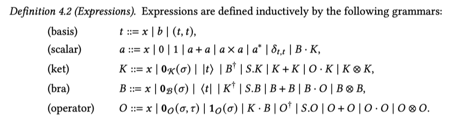
Scalars. Our algorithm has the normalization for scalars, which is different from that in Mathematica. Therefore we use a different set of symbols to represent scalar expressions, with the specified rewriting rules.
In[]:=
{PAIR[t1,t2],CPX[0],a~ADDS~b,DELTA[s,t]}
Out[]=
{PAIR[t1,t2],CPX[0],(ab),}
+
S
δ
s,t
Ket
In[]:=
{ZEROK[T],KET[s],ADJK[b],a~SCRK~k,k1~ADDK~k2,o~MLTK~k,k1~TSRK~k2}
Out[]=
{[T],|s〉,,(ak),(k1k2),(ok),(k1⊗k2)}
0
K
†
K
b
+
K
·
K
K
Operators
In[]:=
{ZEROO[T1,T2],ONEO[T],k~OUTER~b,o1~ADDO~o2}
Out[]=
{[T1,T2],[T],(k⊗b),(o1o2)}
0
O
1
O
P
+
O
Contexts
Contexts
A context preserves the typing information for variables, which is used during type inference. Here it is represented by a List of rules. For example, the following context declares that s is a basis in T1, o is an operator, and k is a ket.
In[]:=
DiracCtx={s->T1,o->OType[T1,T2],k->KType[T2]}
Out[]=
{sT1,oOType[T1,T2],kKType[T2]}
Extended Language DNE
Extended Language DNE
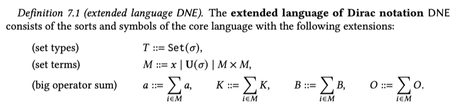
Our language is also able to reason about summation.
Set Types
In[]:=
{SetType[sigma]}
Out[]=
{SetType[sigma]}
Set Terms
In[]:=
{USET[sigma],M1~SETPROD~M2}
Out[]=
{USET[sigma],SETPROD[M1,M2]}
Big Operator Sum
In[]:=
SUMK[i,M,a]
Out[]=
SUMK[IDX[{i,M}],a]
User Language
Dirac notation is a convenient tool because the strict typing can be inferred from the context. This allows us to express the calculation using the application symbol, which is usually omitted.
We designed the user language with nice syntax to recover this mechanism.
We designed the user language with nice syntax to recover this mechanism.
In[]:=
(〈i|∘A∘|j〉)∘(|i〉⊗|j〉)
Out[]=
(〈i|∘A∘|j〉)∘(|i〉⊗|j〉)
Methods
These are the methods defined in our package for Dirac notation reasonings.
DiracParse
DiracParse
Based on the context, transform the user language into the explicit internal language by type inference.
In[]:=
DiracCtx={i->T1,j->T2,A->OType[T1,T2]};DiracParse[(〈i|∘A∘|j〉)∘((|i〉⊗|j〉)∘〈i|)]
Out[]=
((〈i|(A|j〉))((|i〉⊗|j〉)⊗〈i|))
·
S
·
K
K
P
In[]:=
DiracParse[((〈i|∘A)∘|j〉)∘((|i〉⊗|j〉)∘〈i|)]
Out[]=
(((〈i|A)|j〉)((|i〉⊗|j〉)⊗〈i|))
·
B
·
S
K
P
Decide the equivalence.
In[]:=
DNEqQ[(〈i|∘A∘|j〉),((〈i|∘A)∘|j〉)]
Out[]=
True
DNNorm
DNNorm
Parse the user language, check the typing and normalize the Dirac expression according to the context.
In[]:=
DiracCtx={s->T1,t->T2};expr=(KET[s]~OUTER~BRA[s])~MLTK~KET[s]
Out[]=
((|s〉⊗〈s|)|s〉)
P
·
K
In[]:=
DNNorm[expr]
Out[]=
|s〉
An expression with illegal typing.
In[]:=
DNNorm[KET[s]~DOT~BRA[t]]
Out[]=
Hold[Throw[{Type Checking Error: ,Private`DOTTyping[KType[T1],BType[T2]],Context: ,{sT1,tT2}}]]
DNEqQ
DNEqQ
Apply DNNorm to the two terms, and use further techniques to decide whether they are equivalent.
In[]:=
DiracCtx={j->T1,M->OType[T1,T2],i->T2};expr1=BRA[i]~DOT~(ADJO[M]~MLTK~KET[j])expr2=CONJS[BRA[j]~DOT~(M~MLTK~KET[i])]
Techniques, Tricks and Facts
Variables with Subscripts
Variables with Subscripts
Variables with subscripts, which is pervasive in the reasoning, is considered and represented by functions.
Flexible Symbol Definitions
Flexible Symbol Definitions
MMA provides flexible and convenient symbol definitions in the field. We can make use of it to define new symbols for Dirac notations incrementally.
Example: defining the trace (some symbols for dynamic typing are involved here)
In fact, we have a list of definitions used in our example list:
Stepwise Investigation by our Preliminary Example
The Problem Setting
The Problem Setting
The DiracDec Encoding
The DiracDec Encoding
Progress by Manual Operation
Progress by Manual Operation
Expand the MMA definition and parse the user language
Expand the MMA definition and parse the user language
Make rewritings
Make rewritings
push symbols into the big-op
decompose the product
calculating FST and SND
the normal form of LHS
normal form of RHS
The algorithm inserts orthogonal basis when necessary.
Checking the equivalence
Checking the equivalence
The two results are equivalent with respect to the substitution of the bound variables.
This is acknowledged by a special restricted unification.
This is acknowledged by a special restricted unification.
Verifying one equation in HHL algorithm
This is one step in the verification of the HHL algorithm. HHL is a famous quantum algorithm for solving linear algebra equations, and the verification is conducted using quantum Hoare logic. This step describes the change of state assertion after applying the inverse quantum fourier transform.
Parameterized Quantum Circuits
It is an example of verifying the equivalence of two parameterized quantum circuits in the symbolic way. Mathematica’s ability to decide scalar equivalence (cos, sin)
is utilized here. It takes one minute to run this example.
is utilized here. It takes one minute to run this example.
Explanation of the Algorithm
We decide the equivalence of Dirac notation by term rewriting. Term rewriting normalize the term by matching and rewriting using a set of rules, and Mathematica has native support for the procedure.
Part of the rewriting rules are displayed here:
ADJK/ADJB
ADJK/ADJB
These are the rules to reduce adjoint (conjugate transpose) on terms of ket, bra and operator.
Sum
Sum
Rules about Sum involve managing the bound variable, and are therefore more complicated.
CITE THIS NOTEBOOK
CITE THIS NOTEBOOK
DiracDec package: automating equational proofs in Dirac notation
by Yingte Xu, Gilles Barthe & Li Zhou
Wolfram Community, STAFF PICKS, February 11, 2025
https://community.wolfram.com/groups/-/m/t/3392316
by Yingte Xu, Gilles Barthe & Li Zhou
Wolfram Community, STAFF PICKS, February 11, 2025
https://community.wolfram.com/groups/-/m/t/3392316