Full code
Full code
Curve
Curve
Branch Points and Differentials
Branch Points and Differentials
Contour Γ
Contour Γ
In[]:=
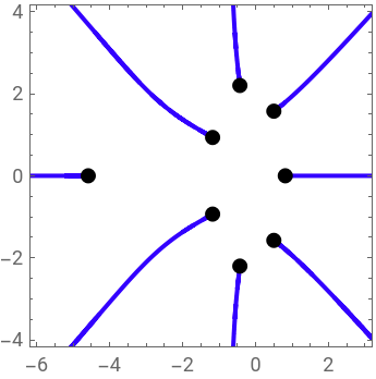
ΔContColor=RGBColor[0.2,0,1];BPPlot=Graphics[Table[{PointSize[Large],Black,Point[{Re[BPs[[k]]],Im[BPs[[k]]]}]},{k,1,Length[BPs]}],Axes->True,PlotRange{{-10,10},{-10,10}},Axes->False];ZeroArgΔ=ContourPlot[Arg[DiscrSF[Rex+IImx]]==0,{Rex,-10,10},{Imx,-10,10},ContourStyle{ΔContColor,Thick},PlotPoints100];Show[ZeroArgΔ,BPPlot,PlotRange->{{-6,3},{-4,4}}]
Out[]=
Solutions for y
Solutions for
y
y Values
y Values
Contour Υ
Contour Υ
In[]:=
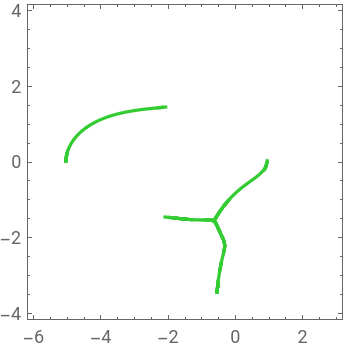
ΥPContColor=RGBColor[{0.2,0.8,0.2}];ZeroArgΥp=ContourPlot[Arg[Υp[Rex+IImx]]==0,{Rex,-6,3},{Imx,-4,4},ContourStyle->ΥPContColor,PlotPoints150]
Out[]=
Density plots of argya
Density plots of
arg
y
a
In[]:=
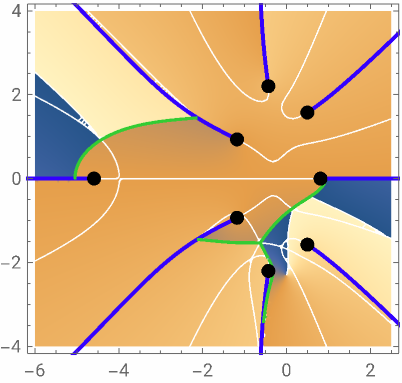
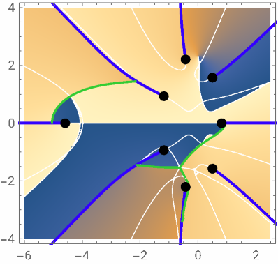
DensArgyP1=DensityPlot[Arg[ySolP1[Rex+IImx]],{Rex,-6,2.5},{Imx,-4,4},PlotLegendsAutomatic,PlotPoints->70];DensArgyP2=DensityPlot[Arg[ySolP2[Rex+IImx]],{Rex,-6,2.5},{Imx,-4,4},PlotLegendsAutomatic,PlotPoints->70];DensArgyP3=DensityPlot[Arg[ySolP3[Rex+IImx]],{Rex,-6,2.5},{Imx,-4,4},PlotLegendsAutomatic,PlotPoints->70];
In[]:=
Show[DensArgyP1,ZeroArgΔ,ZeroArgΥp,BPPlot,PlotRange->{{-6,2.5},{-4,4}},AspectRatio->Automatic]
Out[]=

In[]:=
Show[DensArgyP2,ZeroArgΔ,ZeroArgΥp,BPPlot,PlotRange->{{-6,2.5},{-4,4}},AspectRatio->Automatic,PlotLegendsAutomatic]
Out[]=
In[]:=
Show[DensArgyP3,ZeroArgΔ,ZeroArgΥp,BPPlot,PlotRange->{{-6,2.5},{-4,4}},AspectRatio->Automatic,PlotLegendsAutomatic]
Out[]=
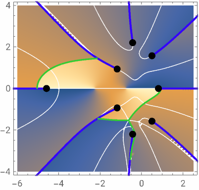
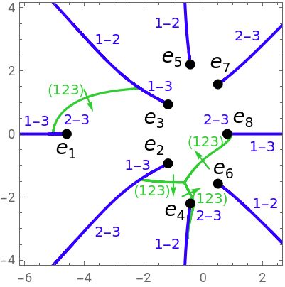
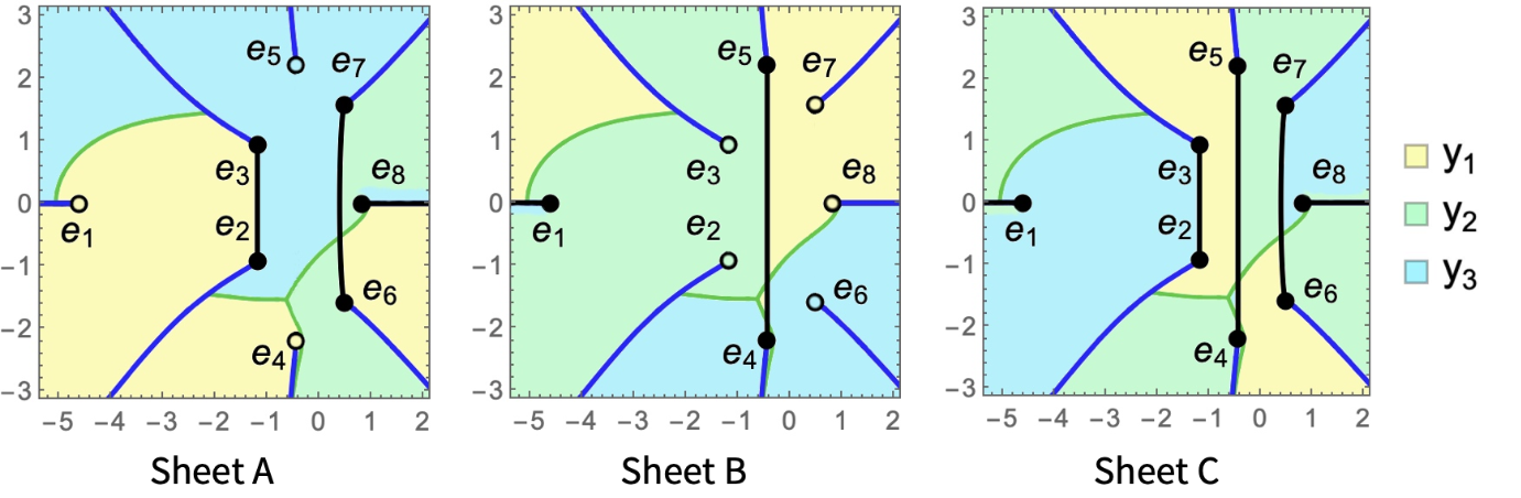
Thelistofconnectionsa-bfromthedensityplotsis
e 1 | e 2 | e 3 | e 4 | e 5 | e 6 | e 7 | e 8 |
1-3 | 2-3 | 1-2 | 1-2 | 1-2 | 1-2 | 2-3 | 1-3 |
Cuts
Cuts
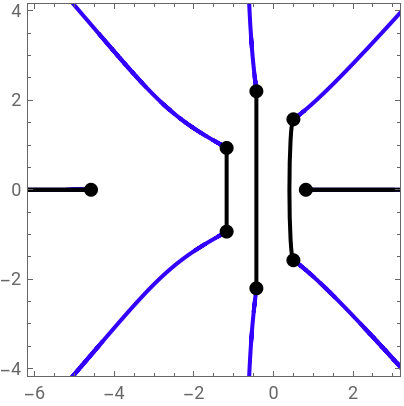
ContoursΓandΥwithconnectionof
y
a
In[]:=
LCut=ContourPlot[Arg[DiscrSF[Rex+IImx]]==0,{Rex,-7,-4},{Imx,-0.5,0.5},ContourStyle->{Thick,Black}];RCut=ContourPlot[Arg[DiscrSF[Rex+IImx]]==0,{Rex,0.8,3},{Imx,-0.5,0.5},ContourStyle->{Thick,Black}];BPcuts=Graphics[{Thick,Black,Line[{{Re[BPs[[2]]],Im[BPs[[2]]]},{Re[BPs[[3]]],Im[BPs[[3]]]}}]}],Graphics[{Thick,Black,Line[{{Re[BPs[[4]]],Im[BPs[[4]]]},{Re[BPs[[5]]],Im[BPs[[5]]]}}]}],GraphicsBlack,Thick,CircleRe[BPs[[6]]+BPs[[7]]],Im[BPs[[6]]+BPs[[7]]],0.1,Abs[BPs[[6]]-BPs[[7]]],Pi,Pi,Graphics[{Thick,Black,Line[{{-10,0},{Re[BPs[[1]]],Im[BPs[[1]]]}}]}],Graphics[{Thick,Black,Line[{{Re[BPs[[8]]],Im[BPs[[8]]]},{10,0}}]}];
1
2
1
2
1
2
1
2
3
2
In[]:=
Show[ZeroArgΔ,BPPlot,BPcuts,LCut,RCut,PlotRange->{{-6,3},{-4,4}}]
Out[]=
First and Second Kind Periods
First and Second Kind Periods
Riemann surface
Riemann surface
Riemannsurfacewithcuts(black),andcontoursΓ(blue)andΥ(green)
Continuouspaththroughallbranchpoints(orange,dashed),andsimplerpathγ,obtainedbycontinuousdefirmationof(orange,solid)
γ
a
γ
First Kind Period matrices
First Kind Period matrices
-Periods
Vector of Riemann constants
Vector of Riemann constants
Computation of ℘ - Functions
Computation of ℘ - Functions
JIP: Example 3a
JIP: Example 3a
JIP: Example 3b
JIP: Example 3b
CITE THIS NOTEBOOK
CITE THIS NOTEBOOK
Uniformization of a genus 3 trigonal curve
by Julia Bernatska
Wolfram Community, STAFF PICKS, August 20, 2024
https://community.wolfram.com/groups/-/m/t/3252458
by Julia Bernatska
Wolfram Community, STAFF PICKS, August 20, 2024
https://community.wolfram.com/groups/-/m/t/3252458