ABSTRACT (original article): Persistent currents circulate continuously without requiring external power sources. Here, we extend their theory to include dissipation within the framework of non-Hermitian quantum Hamiltonians. Using Green’s function formalism, we introduce a non-Hermitian Fermi-Dirac distribution and derive an analytical expression for the persistent current that relies solely on the complex spectrum. We apply our formula to two dissipative models supporting persistent currents: (i) a phase-biased superconducting-normal-superconducting junction; (ii) a normal ring threaded by a magnetic flux. We show that the persistent currents in both systems exhibit no anomalies at any emergent exceptional points, whose signatures are only discernible in the current susceptibility. We validate our findings by exact diagonalization and extend them to account for finite temperatures and interaction effects. Our formalism offers a general framework for computing quantum many-body observables of non-Hermitian systems in equilibrium, with potential extensions to non-equilibrium scenarios. CITATION (original article): Pei-Xin Shen, Zhide Lu, Jose Lado, and Mircea Trif, Non-Hermitian Fermi-Dirac Distribution in Persistent Current Transport, Phys. Rev. Lett. 133, 086301 (2024). https://doi.org/10.1103/PhysRevLett.133.086301
Introduction
Introduction
This notebook accompanies the Letter titled Non-Hermitian Fermi-Dirac Distribution in Persistent Current Transport and provides a comprehensive exploration of dissipation within the framework of non-Hermitian quantum Hamiltonians. We introduce the non-Hermitian Fermi-Dirac distribution via Green’s function formalism, offering both analytical derivations and numerical verifications to extend the understanding of persistent currents in phase-biased SNS junctions and mesoscopic rings. Beyond supporting the findings of the Letter, this notebook includes detailed derivations, visualizations, and numerical verifications of key concepts, such as the continuity of quantum many-body observables at exceptional points and the construction of non-Hermitian effective Hamiltonians. This notebook serves as a valuable resource for researchers investigating the interplay between dissipation, non-Hermitian dynamics, and quantum transport.
Non-Hermitian Fermi-Dirac Distribution in Equation (8)
Non-Hermitian Fermi-Dirac Distribution in Equation (8)
In this chapter, we delve into the detailed derivation, visualization, and asymptotic behavior of the non-Hermitian Fermi-Dirac distribution as formulated in Equation (8) of the accompanying Letter.
Derivation
Derivation
The derivation in this section involves detailed analysis of the integrand poles, supported by useful identities, along with contour integration in the complex plane.
Integrand Poles
Integrand Poles
We begin by analyzing the poles of the integrand in Equation (S14):
In[]:=
Clear["Global`*"];integrand=;FullSimplify@FunctionPoles[integrand,ω]
1
Exp[βω]+1
1
ω-ε
Out[]=
{ε,1},,1
Useful Identities
Useful Identities
Lower Half
Lower Half
We first visualize the integrand in the lower half of the complex plane.
In[]:=
Block[{β=1,R=10,ε=1-},Show[ComplexPlot[integrand,{ω,-R-R,+R+R},ColorFunction->"MaxAbs"],RegionPlot@Disk[{0,0},R,{π,2π}],ImageSize->Medium]]
Out[]=
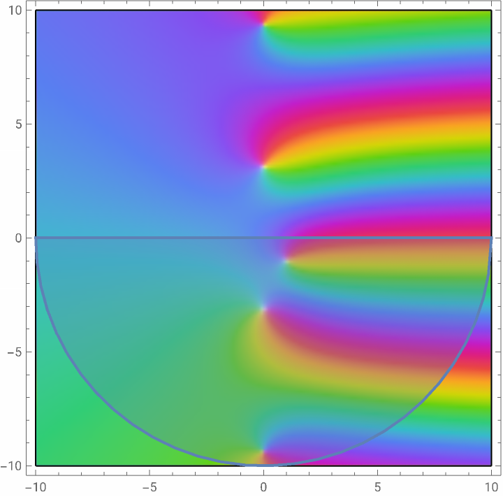
The residue of the complex eigenvalue in the lower half of the complex plane is calculated as:
In[]:=
FullSimplify[-2πResidue[integrand,{ω,ε}]]
Out[]=
-
2π
1+
βε
Additionally, we calculate the residue of the singularity along the negative imaginary axis as:
In[]:=
FullSimplify@Block{M=6},Sum[-2πResidue[integrand,{ω,(m-1/2)2π/β}],{m,-M+1,0}]==-Sum,{m,1,M}==-PolyGamma+M+--PolyGamma+-
-1
+m--
1
2
βε
2π
1
2
βε
2π
1
2
βε
2π
Out[]=
True
This confirms the equivalence of the sums involving residues and digamma functions.
Upper Half
Upper Half
Similarly, we visualize the integrand in the upper half of the complex plane.
In[]:=
Block[{β=1,R=10,ε=1-},Show[ComplexPlot[integrand,{ω,-R-R,+R+R},ColorFunction->"MaxAbs"],RegionPlot@Disk[{0,0},R,{0,π}],ImageSize->Medium]]
Out[]=
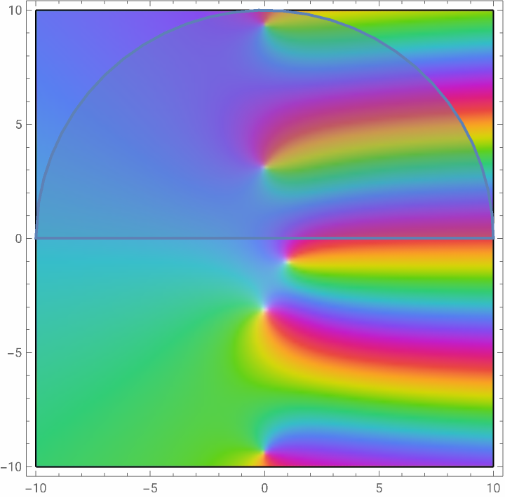
The residue of the singularity along the positive imaginary axis is calculated as:
In[]:=
FullSimplify@Block{M=6},Sum[+2πResidue[integrand,{ω,(m-1/2)2π/β}],{m,1,+M,1}]==-Sum,{m,1,M}==-PolyGamma+M++-PolyGamma++
-1
+m-+
1
2
βε
2π
1
2
βε
2π
1
2
βε
2π
Out[]=
True
Again, this confirms the validity of the derived expressions with digamma functions.
Average Two Contours
Average Two Contours
Visualization
Visualization
In this section, we visualize the derived non-Hermitian Fermi-Dirac distribution under different temperature conditions: and , which corresponds to Figure 3(c) in the main text.
T0
T≠0
T0
T0
We define the non-Hermitian Fermi-Dirac distribution at zero temperature , and verify that the distribution function is analytic in the lower half of the complex plane.
T0
In[]:=
Clear["Global`*"];feff[ε_]:=-Log[ε];FunctionAnalytic[{feff[ε],Im[ε]<0},ε,]
1
π
Out[]=
True
We generate a 3D plot that visualizes the imaginary part of the non-Hermitian Fermi-Dirac distribution at zero temperature. The axes represent the real and imaginary parts of the complex energy ε.
In[]:=
Block{ε=rExp[ϕ]},ShowGraphics3DArrowheads[0.05],Arrow[{{0,0,0},{1.2,0,0}}],Text["Re ε",{1.1,-0.2,0}],Arrow[{{0,0,0},{0,-0.9,0}}],Text["Im ε",{-0.2,-0.8,0}],Arrow[{{0,0,0},{0,0,1.2}}],Text["Θ(-ϵ)",{0.3,0,0.6}],Text"-Im[ln(ε)]",{0,0,1.3},Text["Im[(ε)]",{-0.5,0,0.5}],Boxed->False,ViewPoint->{5,-10,5},AspectRatio->23,BaseStyle->{FontFamily->"Times",FontSize->24},ParametricPlot3D[{Re@ε,Im@ε,Im@feff[ε]},{r,0,1},{ϕ,π,2π},PlotStyle->Opacity[0.5],Mesh->None,ColorFunction(Hue[#5]&),Axes->False],ParametricPlot3D[{ϵ,0,HeavisideTheta[-ϵ]},{ϵ,-1,1},PlotStyle->{Black,Dashing[0.012],Thickness[0.01]},ExclusionsStyle{{Black,Dashing[0.015],Thickness[0.01]},Black}],ParametricPlot3D[{x,0,z},{x,-1,1},{z,0,1},Mesh->None,PlotStyle->Directive[Gray,Opacity[0.1]]],ImageSize->350,Method->{"ShrinkWrap"->True}
1
π
f
eff
Out[]=

We create a 3D plot to visualize the imaginary part of the non-Hermitian Fermi-Dirac distribution at finite temperature. The axes again represent the real and imaginary parts the complex energy ε.
Asymptotic Behavior
Asymptotic Behavior
Current Continuity at Exceptional Points
Current Continuity at Exceptional Points
In this chapter, we examine the continuity of quantum many-body observables—persistent currents—at exceptional points in non-Hermitian systems. We begin with a toy model to demonstrate the general principles, followed by an in-depth analysis based on the derivations in Section II-D of the Supplemental Material, focusing on the behavior of the non-Hermitian Fermi-Dirac distribution and free energy at both zero and finite temperatures.
Toy Model
Toy Model
In this section, we provide technical details regarding the continuity of many-body observables for a non-Hermitian toy model at exceptional points, as discussed in the blog titled Quantum many-body observables in equilibrium are continuous at exceptional points.
Section II-D in Supplemental Material
Section II-D in Supplemental Material
This section addresses the continuity of current at exceptional points, as discussed in Section II-D of the Supplemental Material. The key focus is on the behavior of the non-Hermitian Fermi-Dirac distribution and the associated free energy, particularly near exceptional points where the system’s wavefunctions coalesce.
Non-Hermitian Effective Hamiltonian
Non-Hermitian Effective Hamiltonian
This chapter elucidates the construction of a non-Hermitian effective Hamiltonian for a fermionic reservoir. It covers the usage of the Green’s function and its application to self-energy calculations, as detailed in Section I of the Supplemental Material.
Green’s Function of a Fermionic Reservoir
Green’s Function of a Fermionic Reservoir
We begin by presenting the analytical expressions for the Green’s function of a fermionic reservoir. This Green’s function is essential for understanding the system’s behavior, particularly regarding the non-Hermitian features introduced by the reservoir.
Numerical Verification
Numerical Verification
The above plot compares the real and imaginary parts of the Green’s function calculated numerically with those derived analytically, validating the consistency between the two methods.
Edge Green’s Function for Self-Energy
Edge Green’s Function for Self-Energy
Finally, we visualize the edge Green’s function, which is pivotal for determining the self-energy corrections, as indicated by Equation (S5) and applied in Equation (S10) of the Supplemental Material.
The above plots demonstrate the excellent agreement between the analytical expression and the numerical results.
Conclusion
Conclusion
In this notebook, we have explored the effects of dissipation on persistent currents in quantum many-body systems, using a newly introduced non-Hermitian Fermi-Dirac distribution. The combination of analytical derivations and numerical verifications presented here provides a robust framework for calculating persistent currents in non-Hermitian systems, particularly in phase-biased SNS junctions and normal mesoscopic rings. Our results confirm that quantum many-body observables in equilibrium remain continuous and exhibit no anomalies at exceptional points, underscoring the validity of the non-Hermitian approach. The notebook not only supports the findings of our Letter but also offers valuable tools for investigating non-Hermitian effects in both equilibrium and non-equilibrium quantum systems.
CITE THIS NOTEBOOK
CITE THIS NOTEBOOK
Non-Hermitian Fermi-Dirac Distribution in Persistent Current Transport
by Pei-Xin Shen, Zhide Lu, Jose L. Lado, and Mircea Trif
Wolfram Community, STAFF PICKS, August 27, 2024
https://community.wolfram.com/groups/-/m/t/3258109
by Pei-Xin Shen, Zhide Lu, Jose L. Lado, and Mircea Trif
Wolfram Community, STAFF PICKS, August 27, 2024
https://community.wolfram.com/groups/-/m/t/3258109