CITE THIS NOTEBOOK: Pairs Trading: terminology and implementation by Jonathan Kinlay. Wolfram Community JAN 23 2023.
Chapter 5: Pairs Trading. An excerpt from the from the forthcoming book “Equity Analytics” by Jonathan Kinlay.
Chapter 5: Pairs Trading. An excerpt from the from the forthcoming book “Equity Analytics” by Jonathan Kinlay.
Pairs trading is a market neutral trading strategy that involves buying and selling two highly correlated financial instruments simultaneously. The idea is to profit from the difference in price movements between the two instruments. Pairs trading is often used in the stock market, but can also be applied to other markets such as futures and options. The strategy is based on the idea that while individual stocks may be affected by company - specific or market - wide events, the relative relationship between two highly correlated stocks will remain relatively stable over time.
Pairs trading involves applying statistical and mathematical techniques to identify and analyze the correlation and co - movement between two financial instruments . Some of the terminology that commonly arises in this context includes:
◼
Statistical Arbitrage : This technique involves analyzing the statistical properties of the price movements of the two or more related instruments in order to identify any mispricing or deviation from the normal relationship between them.
◼
Correlation Analysis : This technique involves calculating the correlation coefficient between the two instruments in order to determine the strength and direction of the relationship between them.
◼
Cointegration Analysis : This technique involves analyzing the long - term relationship between the two instruments to determine if they are cointegrated, meaning that they move together over time.
◼
Spread Trading : This technique involves calculating the ratio or difference between the prices of the two instruments and then trading based on the movements of this spread.
◼
Risk Management : Pairs traders use various risk management techniques to minimize their losses . They typically use stop - loss orders and other techniques to limit their downside risk.
◼
Backtesting : Pairs traders use historical data to test the performance of their trading strategy,tune the strategy parameters and make adjustments to the strategy if necessary.
Pairs Trading Coke vs. Pepsi with the Kalman Filter
To illustrate the application of the various techniques used in developing a pairs strategy we will choose the stock pair {,}, i.e. Pepsi and Coke.
Stock Selection & Parameter Settings
Stock Selection & Parameter Settings
In[]:=
timeStep={1,"BusinessDay"};startDate=DateObject[{2018,1,2},"Day"];endDate=DateObject[{2022,12,31},"Day"];initDate=NextDate[DatePlus[startDate,{-6,"Month"}],"BusinessDay"];symbols={"PEP","KO"};stocks=Entity["Equities",#]&/@symbols;maxTrades=1;portfolioUnits=1000;slippage=AssociationThread[symbols->(Quantity[#,"US Dollars"]&/@{0.01,0.01})];commission=Quantity[0.005,"US Dollars"];
Price and Return Data
Price and Return Data
We first extract the price and returns series for the two stocks from the Entity Store, over the period specified in the strategy parameters above, as follows:
In[]:=
tsPriceSeries=<|Association[GetSymbol[#]->TimeSeriesWindow[#["Historical Data"]["Price Data","Daily Prices"],{initDate,endDate}]&/@stocks]|>
Out[]=
PEPTimeSeries,KOTimeSeries


We will use log-returns rather than the daily returns since, as we have seen, the log transform tends to produce a more stationary time series:
In[]:=
tsReturnsSeries=Differences[Log[#["PathComponent","Close"]]]&/@tsPriceSeries
Out[]=
PEPTimeSeries,KOTimeSeries


Modeling the Price Co-Movements
Modeling the Price Co-Movements
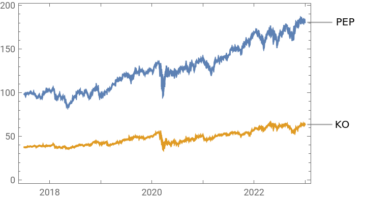
The Pepsi and Coke price series are clearly highly correlated:
In[]:=
DateListPlot[#["PathComponent","Close"]&/@Values[tsPriceSeries],PlotLabels->symbols]
Out[]=
In[]:=
Correlation[Transpose@Join[#["PathComponent","Close"]["Values"]&/@Values[tsPriceSeries]]]//MatrixForm
Out[]//MatrixForm=
1. | 0.960282 |
0.960282 | 1. |
Correlation & Cointegration of the Returns Series
Correlation & Cointegration of the Returns Series
In the ensuing analysis we will focus on the returns series for both stocks. This has the advantage of ensuring stationarity in the series used for analysis. Again, we see a very high level of correlation between the two stock return processes:
In[]:=
ListPlot[Transpose@Join[#["Values"]&/@Values[tsReturnsSeries]]]
Out[]=
In[]:=
Correlation[Transpose@Join[#["Values"]&/@Values[tsReturnsSeries]]]//MatrixForm
Out[]//MatrixForm=
1. | 0.748218 |
0.748218 | 1. |
Johansen Test for Cointegration
Johansen Test for Cointegration
Cointegration is a statistical property of a collection of time series, which suggests that they are related in such a way that a linear combination of them is stationary. Cointegration is often used in econometrics and finance to model stable, long - term relationships between variables.
A spurious correlation is a statistical relationship between two variables that appear to be related but are not actually causally related. This type of correlation can occur due to chance or due to a third variable that is not being considered.
Co-integration is regarded as a more reliable gauge of the relationship between series than correlation, as it seeks to account for the presence of such common factors.
A spurious correlation is a statistical relationship between two variables that appear to be related but are not actually causally related. This type of correlation can occur due to chance or due to a third variable that is not being considered.
Co-integration is regarded as a more reliable gauge of the relationship between series than correlation, as it seeks to account for the presence of such common factors.
Examples of cointegrated series in finance include :
◼
The relationship between stock prices and dividends
◼
The relationship between interest rates and bond prices
◼
The relationship between exchange rates of two currencies
Examples of cointegrated series in economics include :
◼
The relationship between GDP and unemployment
◼
The relationship between inflation and money supply
◼
The relationship between housing prices and rental rates .
The typical workflow in pairs trading is to test for cointegration between the pair of correlated processes using a procedure developed by Engle and Granger, or a more comprehensive test developed by Soren Johansen.
The Johansen test evaluates whether there are at least r cointegrating relationships between between k different time series and is more general than the Engle-Granger procedure. The test comes in two forms, the first using the trace statistic, the second the eigenvalue. The null hypothesis is that the number of cointegration vectors is r = r* < k, vs. the alternative that r = k. Testing proceeds sequentially for r* = 1, 2, etc. and the first non-rejection of the null is taken as an estimate of r.
Here we would reject the null hypothesis in the case of r <=1, concluding (with 99% confidence) that there is at least one cointegrating relationship between the two stock returns processes.
Here we would reject the null hypothesis in the case of r <=1, concluding (with 99% confidence) that there is at least one cointegrating relationship between the two stock returns processes.
In[]:=
PrintStats[JohansenTest[Join[#["Values"]&/@Values[tsReturnsSeries]],2,0]]
NULL Trace Statistic Crit 90% Crit 95% Crit 99%
r<=0 |
r<=1 |
1122.65 |
515.781 |
10.4741 | 12.3212 | 16.364 |
2.9762 | 4.1296 | 6.9406 |
NULL Eigen Statistic Crit 90% Crit 95% Crit 99%
r<=0 |
r<=1 |
606.873 |
515.781 |
9.4748 | 11.2246 | 15.0923 |
2.9762 | 4.1296 | 6.9406 |
Kalman Filter Spread Model
Kalman Filter Spread Model
The Kalman filter is a mathematical algorithm that uses a series of measurements and predictions to estimate the state of a system over time. It is commonly used in control systems, navigation systems, and signal processing. In the context of pairs trading, the Kalman filter can be used to estimate the spread between the prices of two correlated financial assets, such as stocks.
If and are non-stationary returns processes with order of integration d=1, then a linear combination of them must be stationary for some value of β and. In other words, the spread:
x
t
y
t
μ
t
y
t
βx
t
μ
t
is a stationary process.
If we knew β , we could just test the spread for stationarity with something like a Dickey–Fuller test. But because β is unknown we have to estimate it using linear regression, or some other technique.
If we knew β , we could just test the spread for stationarity with something like a Dickey–Fuller test. But because β is unknown we have to estimate it using linear regression, or some other technique.
In this example we model the relationship between the two stocks using a Kalman filter, which dynamically estimates the regression coefficient , which represents the “state” of the linear relationship between the two returns processes as it changes over time. So in this case the model is:
β
t
y
t
β
t
x
t
μ
t
where the regression coefficient is updated at each timestep.
The Equities Entity Store has a suite of functions to model pairs relationships using a variety of statistical techniques, including the Kalman filter.
β
t
The Equities Entity Store has a suite of functions to model pairs relationships using a variety of statistical techniques, including the Kalman filter.
The Importance of Stationarity in Finance
The Importance of Stationarity in Finance
It is common practise these days to stress the limitations of the assumption of Normality as applied to asset returns processes in standard economic models. The phenomenon of “fat tails” - the tendency to observe extremely large, positive or negative values much more frequently in an empirical dataset than would be expected if the data were Normally distributed - has been thoroughly documented. The assumption of Normality is important, as it simplifies the procedure for statistical inference. Conversely, if the process we are studying is non-Gaussian it may invalidate certain statistical tests and, in extreme cases, our entire model. Usually, however, we are able to overlook or work around the non-Gaussian behavior of the process without incurring too great a penalty; in other cases we might transform the data to produce something closer to a Gaussian-distributed dataset, or employ a “fudge factor” to make adjustments to our model, as is the case with the volatility skew in the Black-Scholes option pricing framework.
Stationarity is another important feature of random processes that greatly simplifies econometric modelling. Econometricians will seek to achieve stationarity in a time series before going on to model it, perhaps by differencing, or applying logs or other data transforms. This makes the series much more tractable for modeling purposes; but stationarity also has real, economic significance too.
To understand why, lets consider a stationary ARMA process:
Stationarity is another important feature of random processes that greatly simplifies econometric modelling. Econometricians will seek to achieve stationarity in a time series before going on to model it, perhaps by differencing, or applying logs or other data transforms. This makes the series much more tractable for modeling purposes; but stationarity also has real, economic significance too.
To understand why, lets consider a stationary ARMA process:
In[]:=
stationaryproc=ARMAProcess[0,{.1},{0.3},1];WeakStationarity[stationaryproc]
Out[]=
True
Now let' s generate a time series of observations from the process and plot them.
In[]:=
stationarydata=RandomFunction[stationaryproc,{0,10^3}]
Out[]=
TemporalData

In[]:=
ListPlot[stationarydata,Filling->Axis]
Out[]=
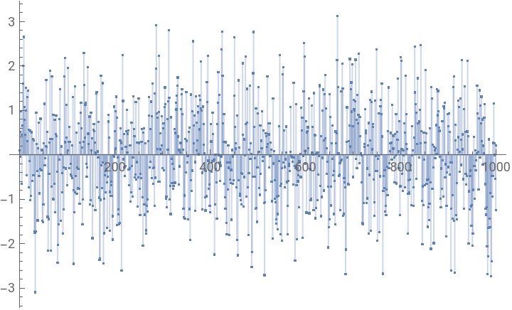
Suppose that this data represents the spread between two stocks. Let’s look at how the spread evolves through time:
As you can see, although the spread periodically moves quite far away from its mean (close to zero in this case), it always eventually reverts to that level. How far away it is likely to move, and how quickly it reverts to its mean, are dependant on the characteristics of the underlying process. But the point is: if the spread is a stationary process then it will revert to its mean eventually, because both the mean and variance of the process are constant. So if we buy the spread when it is low (or negative) and sell it when it is high, we are likely to make money, over the long term.
Now lets look at some sample data from a non-stationary process:
Again, assuming the data represents the spread between two stocks, you can see that, because the underlying process is non-stationary, the spread can wander arbitrarily far away from its mean. If we try to sell such a spread when it is high, or buy when it is low, we could easily suffer catastrophic losses as the spread continues to widen, or narrow.
So the issue of stationarity is of vital significance in the context of pairs trading, which works on the assumption that the spread is stationary and therefore mean-reverting.
Unit Roots
Unit Roots
A unit root is a statistical concept used in time series analysis to describe a non - stationary time series that can be made stationary through the use of a first - differencing transformation . A time series with a unit root is said to be integrated of order 1, or I (1) for short. The most common unit root test is the Augmented Dickey - Fuller test, which is used to determine whether a time series has a unit root.
In reality, we have no way of knowing the precise form of the process underlying a time series like a spread - all we have is a sample of data. So how do we determine whether the process is stationary, or not? Fortunately there are a series of tests that can be applied to determine the answer. The UnitRootTest function applies the Dickey-Fuller and Phillips-Perron F and T tests to determine the likelihood that the process contains a unit root and is therefore non-stationary (the null hypothesis). More specifically, we test for a unit root in a model of the form:
where α is the constant offset, β is a linear drift, and r is the order of the autoregressive model.
In cases where, for example, the data represents a time series of stock returns, or a spread, we would normally assume the constant and trend terms are zero and that r = 1. So the model then becomes:
Returning to our illustration, for the stationary data series all four variants of the unit root test convincingly reject the null hypothesis of a unit root, leading us to conclude that the underlying process is stationary, as indeed we know it to be:
On the other hand, for the non-stationary data, none of the test variants rejects the null hypothesis, leading to the correct conclusion that the underlying process is non-stationary.
Unfortunately, however, life is the real world is rarely as simple as this. Unit Root tests have quite low power and are often unable to distinguish correctly between a process that is non-stationary, but close to being stationary vs. one that is stationary, but close to being non-stationary. In simple terms, when we are looking at the data from a pairs spread, it is often very difficult to determine for sure whether the underlying process is truly stationary and that the spread will consequently revert to the mean, or non-stationary, and is therefore unsuitable for trading. Indeed, we often find cases where statistical tests indicate that the process is stationary, but the rate of mean reversion is so slow that a pairs strategy is likely to go through prolonged and very uncomfortable drawdowns before turning profitable.
For these reasons a pairs trading strategy will typically incorporate a stop loss that will exit the trade if the spread continues to move in the wrong direction: the trader just can’t afford to take the risk that, despite indications to the contrary, the spread is non-stationary and/or has broken down - meaning that its characteristics have changed in some fundamental way, rendering historical analysis moot.
A further safety measure that many pairs trading strategists adopt is to screen potential pairs trades, selecting only those for which there is some basis in economic reality to suggest that their relationship is likely to be an enduring one. So, for example, the analyst might reject pairs of stocks that belong to different sectors or industries, regardless of how correlated or cointegrated the series might appear. A pair like Coke-Pepsi is likely to pass such a filter due to the fundamental similarities in the two companies and their products; a pair involving a stock like TSLA, on the other hand, would perhaps be unlikely to be chosen because the firm is a recent entrant into the automotive industry and its innovative products are very different to those of incumbents, who continue to rely on legacy products for the majority of their revenues.
For these reasons a pairs trading strategy will typically incorporate a stop loss that will exit the trade if the spread continues to move in the wrong direction: the trader just can’t afford to take the risk that, despite indications to the contrary, the spread is non-stationary and/or has broken down - meaning that its characteristics have changed in some fundamental way, rendering historical analysis moot.
A further safety measure that many pairs trading strategists adopt is to screen potential pairs trades, selecting only those for which there is some basis in economic reality to suggest that their relationship is likely to be an enduring one. So, for example, the analyst might reject pairs of stocks that belong to different sectors or industries, regardless of how correlated or cointegrated the series might appear. A pair like Coke-Pepsi is likely to pass such a filter due to the fundamental similarities in the two companies and their products; a pair involving a stock like TSLA, on the other hand, would perhaps be unlikely to be chosen because the firm is a recent entrant into the automotive industry and its innovative products are very different to those of incumbents, who continue to rely on legacy products for the majority of their revenues.
More broadly, we might regard the “gold standard” for candidates for pairs trading to be, say, a cash-futures pair, such as Treasury Bonds vs. Bond futures. Here, not only are the series both highly correlated and cointegrated, there is an economic principle (the law of one price) that connects the two markets and ensures that the price of related instruments cannot diverge by too much for too long. So in this case the fundamental and statistical rationale for the trade overlap, giving us considerable confidence in it. Of course, the problem is that everyone understand this, so price discrepancies are very quickly arbitraged away. What the strategist seeks, therefore, is a pairs trade with both a cogent economic rationale as well as a compelling statistical relationship, that is not too widely known or understood. One of the benefits of developing pairs trading strategies in equities is that there is a very large universe of potential pairs to choose from: in the Equities Entity Store alone there are approximately as many as 7500^2 ≈ 56 million possibilities to consider.
We will return to the important topic of pairs selection in a later chapter.
Notes
Notes
◼
More on stationarity and unit root tests : Cointegration Breakdown
Implementing the Kalman Filter Model
Implementing the Kalman Filter Model
Returning to our Pepsi-Coke trade, we use the ReturnsTimeSeriesKalman function to create a Kalman filter model producing time-varying estimates of the beta coefficient of the linear relationship between the two stock returns series:
Before proceeding, we first want to test the time series of Zscores for stationarity, as it is these scores that we are going to use to generate signals to trade the spread, on the assumption that it is mean-reverting. All four variants of the UnitRootTest roundly reject the null hypothesis of a unit root, leading us to conclude that the spread is indeed stationary and therefore tradeable:
Trading Signals
Trading Signals
In order to proceed with the implementation and backtesting of our strategy, we first need to process the Zscores and convert them into trading signals. Before doing that, let’s look at the distribution of the Zscores:
Applying a battery of standard tests for Normality, we find that the distribution of the ZScores clearly isn’t Gaussian:
But this is one of those instances in finance where non-Normality doesn’t matter: all that concerns us is that the series is stationary and therefore that the mean and variance are time-invariant and the process is consequently mean reverting.
In the early days of pairs trading it was quite commonplace to make the simplifying assumption that the model residuals followed a Normal distribution: then we might regard a value of +/- 1.96 in the standardized Zscores, corresponding to the 5%-tile and 95%-tile of the Normal distribution, as appropriate levels for entry signals. But there really isn’t any need to make such a heroic assumption. First of all, we know for sure that the distribution of the Zscores from our model is non-Gaussian. Secondly, in the Kalman model you standardize the residuals, not in the usual way by using their estimated standard deviation, but by using the square root of the estimate of the time-varying variance of the system state at each time step. So the overall standard deviation of the Zscores in this example is not 1, but closer to 0.25, as we have shown above.
Either way it doesn’t matter, because the Gaussian assumption is unnecessary; we have empirical data from which we can select suitable entry signals, using appropriate quantiles of the empirical distribution:
In the early days of pairs trading it was quite commonplace to make the simplifying assumption that the model residuals followed a Normal distribution: then we might regard a value of +/- 1.96 in the standardized Zscores, corresponding to the 5%-tile and 95%-tile of the Normal distribution, as appropriate levels for entry signals. But there really isn’t any need to make such a heroic assumption. First of all, we know for sure that the distribution of the Zscores from our model is non-Gaussian. Secondly, in the Kalman model you standardize the residuals, not in the usual way by using their estimated standard deviation, but by using the square root of the estimate of the time-varying variance of the system state at each time step. So the overall standard deviation of the Zscores in this example is not 1, but closer to 0.25, as we have shown above.
Either way it doesn’t matter, because the Gaussian assumption is unnecessary; we have empirical data from which we can select suitable entry signals, using appropriate quantiles of the empirical distribution:
The quantile of the empirical distribution that is used for trade entry signals is one of the system hyperparameters that can be tuned. However, this get perilously close to curve-fitting, in my view. I prefer to select a “sensible” quantile value, even if it isn’t necessarily the optimal level - if the strategy works at all, it should work pretty well across a range of reasonable values, or else it is likely to prove too unreliable out of sample.
In this model, the entry level quantile is determined by the parameter levelSpacing, which I have set to 0.5, slightly less that 2x the standard deviation of the Zscores. This means that a Zscore of -0.5 or less will trigger a long entry signal, while a value of 0.5 or more will trigger a short entry. These values correspond to the 2.3%-tile and 98%-tile of the distribution, respectively:
There is nothing magical about this choice of entry level. You might just as easily have chosen the 5%-tile and 95%-tile levels of the distribution, i.e.
What' s important, however, is that you select a level that produces enough, but not too many trades. If the system generates too few trades it will be difficult to assess its robustness and likelihood of continuing success, going forward. Generating too many trades, on the other hand, may see your profits eviscerated by transaction costs. So the aim should be for an entry level that provides a reasonable balance. For a pairs strategy built using daily data, around one trade per quarter might be an appropriate guideline. If that seems like quite a low number, bear in mind that in a pairs trading system you would typically expect to be trading a universe comprising dozens of stock pairs, which in aggregate will generate multiple trading signals every week.
Trade Exits
Trade Exits
Without wishing to get too deep into the weeds, there are a couple of other choices that need to be made with regard to trading signals. The first is to decide what to do about trade exits. There are various schemes for this. A common approach, which is the one adopted here, is to hold the current position until a signal is received in the opposite direction, a scheme which is known as “stop and reverse”. An equally common alternative is to exit an open position when the Zscore crosses the zero line. This will usually produce a larger number of trades of shorter duration and with lower average profit. The first approach is certainly a little simpler, but there is no compelling argument to be made one way or another.
Repeated Signals / Multiple Entries
Repeated Signals / Multiple Entries
The second choice that needs to be made is what to do about repeated signals, i.e. when a signal that exceeds the threshold level is followed by another signal (in the same direction) that also exceeds the threshold (or an even higher level). The signals may follow one another in sequence, or there may be a delay of several periods between the first and subsequent signals.
The default action of the system in the ZscoreSignals function is to process only the first such signal, but the parameter maxTrades can be configured so that additional signals are considered. More specifically, the total size of the position taken is dependent on (a) the maxTrades parameter value and (b) the magnitude of the signal as a multiple of the levelSpacing parameter. With the value of levelSpacing set to 0.5 and maxTrades set to 2 or higher, the value specified in this example, the system will produce a short trade 2x the default size if a Zscore is encountered that is greater than 1.0 (twice the value of the levelSpacing parameter), while a short trade of 3x the default size is generated for a Zscore value of 1.5, or higher.
The default action of the system in the ZscoreSignals function is to process only the first such signal, but the parameter maxTrades can be configured so that additional signals are considered. More specifically, the total size of the position taken is dependent on (a) the maxTrades parameter value and (b) the magnitude of the signal as a multiple of the levelSpacing parameter. With the value of levelSpacing set to 0.5 and maxTrades set to 2 or higher, the value specified in this example, the system will produce a short trade 2x the default size if a Zscore is encountered that is greater than 1.0 (twice the value of the levelSpacing parameter), while a short trade of 3x the default size is generated for a Zscore value of 1.5, or higher.
Here we set maxTrades = 1 and take only the first signal, ignoring subsequent signals in the same direction as the previous one:
Finally, we truncate the signals time series to the window defined by the start and end date parameters, before moving on to strategy backtesting.
Notes
Notes