Wolfram Cloud Document

This notebook demonstrates basic Kalman filtering -- parameter estimation specifically -- as a functional fold over lists, streams, and asynchronous observables. It exhibits applications from estimating the coefficients of a polynomial to tracking in 2D. It includes a concise redux of Kalman’s theory. It is pedagogical in nature.

FUNCTIONAL: because we write Kalman as a Fold (you might be “functional” if you’re using map, filter, fold, bind, ...). Functional is good because it separates algorithms from transport, storage, timing, and so on. Functional is good because it promotes composition — better code from smaller building blocks. Functional is good because it supports mathematical reasoning & proofs.

REACTIVE: because Kalman takes inputs one at a time, therefore works equally well on iterables as on observables. Reactive is good because exactly the same algorithmic code works on synchronous, asynchronous; offline and online; finite, and infinite collections.

PARAMETER ESTIMATION: because Kalman optimally estimates parameters and states of models. Models predict phenomena like aircraft position and economic trends.

We’ll show that Kalman is functional, reactive least-squares regression. It’s also an instance of a Hidden Markov Model—a model with a memory one back. Hidden Markov models can be expressed as functional folds, e.g., the Viterbi algorithm.

The goal here is instruction, for you to OWN Kalman in your toolbelt, so you can recognize when, where, and how to use it. Owning it in functional, reactive form lets you use it in a variety of settings from the lab to the field with high assurance.

Introduction

Kalman filtering fits in the following matrix of statistical algorithms; all of these are folds. Note the word iteractive is not a misspelling of interactive. Iteractive is dual to reactive. Reactive describes asynchronous push-models wherein data are pushed into procedures, as with observables. Iteractive describes synchronous pull models wherein procedures pull data from sources. This paper will gradually motivate, derive, and demonstrate the highlighted functions.

	Batch	iteractive,reactive	functions
iterator		foreachsubscribe	z=observation
L 0	count=N	count	{z0,z}z0+ 0 z
L 1	mean= - x = 1 N N ∑ i=1 x i	summean	{z1,z}z1+ 1 z {(z0,z1),z} z1+ 1 z z0+ 0 z
L 2	ssr=∑ 2 ( x i - - x )	sumsqrsnaivessrWelford's	{z2,z}z2+ 2 z {(z0,z1,z2),z}(z2+ 2 z )- 2 (z1+ 1 z ) z0+ 0 z {(z0,z1,ssr),z}0if(z00)elsessr+z- z1 z0 z- z1+ 1 z z0+ 0 z
fit	least–squaresregression	KalmanPotterSRIFEKFUKFΣPF...	{(x,P),(z,A)} (K.(z-A.x),P-K.D.  K ) (newx,newP),whereK=P.  A . -1 D D= -1 (I+A.P.  A )

Taxonomy

The following terminology will appear in your reading about Kalman filtering. It is presented here just to show the richness of the field.

Potter = better numerics (Potter is to Kalman as Welford is to naive SSR: don’t subtract squared numbers!)

SRIF = Square-Root Information Filter

U/D = Decomposed Kalman (Thornton, Bierman); another way to avoid squaring

EKF = Extended Kalman Filter (works on non-linear models)

UKF = Unscented Kalman Filter (works on non-Gaussian statistics)

ΣPF = Sigma-Point Filter (generalization of UKF)

Particle Filter = when all else fails (expensive but versatile)

Prerequisite: Folds over Lists, Lazy Lists, and Tasks

Details are in my article on Folds over Lists, Streams, and Asynchronous Observables, https://community.wolfram.com/groups/-/m/t/3074231. This section defines just the expressions we need from that article for this one. Here, we shall fold Kalman accumulators over lists, streams (lazy lists), and observables (asynchronous data sources).

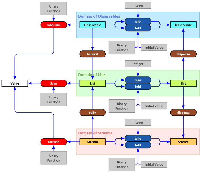
The following figure illustrates the functional symmetries between lists, streams, and observables. All can be processed with higher-order functions like map, filter, and fold.

Lists

In general, a fold takes three arguments: a binary query or accumulation function, a starting value, and a collection of other values. FoldList, in Wolfram, produces all intermediate values and is thus composable with other list-producing operators.

FoldList :: query ⟶ startingValue ⟶ list ⟶ list

See https://community.wolfram.com/groups/-/m/t/3074231 for examples.

repeat :: Expression ⟶ count ⟶ list

We need this below for a tracking example.

In[]:=

repeat[e_,n_Integer]:=Table[e,{n}];matrixMultiply=Dot;

Streams

Represent a stream as a pair of a value and a thunk (procedure of no arguments). The thunk must produce another stream.

We need the infinite stream of integers for the tracking example.

In[]:=

integersFrom[n_Integer]:={n,integersFrom[n+1]&}

take :: stream ⟶ index ⟶ stream

Here’s an operation that takes a finite number of elements from a stream and produces another stream. We need this for examples below.

In[]:=

ClearAll[take];take[stream_]:=take[stream,1];take[_,0]:=Null[];take[Null[],_]:=Null[];take[{v_,thunk_},1]:={v,Null};take[{v_,thunk_},n_Integer/;n>0]:={v,take[thunk[],n-1]&};

takeUntil :: stream ⟶ (value ⟶ Boolean) ⟶ index ⟶ stream

Here’s an operation that takes elements until some predicate evaluates to True, excluding that element. We need this for the tracking example).

In[]:=

ClearAll[takeUntil];takeUntil[Null[],_]:=Null[];takeUntil[{v_,thunk_},predicate_]/;predicate[v]:=Null[];takeUntil[{v_,thunk_},predicate_]:={v,takeUntil[thunk[],predicate]&};

reify :: stream ⟶ list

Reify a stream to a list, rattling out all thunks (this is not tail-recursive; we might have to do better if the stack overflows):

In[]:=

ClearAll[reify];reify[Null[]]:={};reify[{v_,Null}]:={v};reify[{v_,thunk_}]:=Join[{v},reify[thunk[]]];

disperse :: list ⟶ stream

Go the other way

In[]:=

ClearAll[disperse];disperse[{}]:=Null[];disperse[{x_}]:={x,Null};disperse[{v_,xs__}]:={v,disperse[{xs}]&};

foldrStream :: query ⟶ initState ⟶ stream ⟶ stream

Here is a fold for streams with the same signature and semantics as FoldList for Lists. It produces a stream from a stream. We’ll fold Kalman over streams with this.

Observable

An observable is an interface with one method: subscribe. The subscribed unary function will be called for each observation produced by the observable. The unary function is called an observer.

subscribe :: observable ⟶ unaryFunction ⟶ Null

We model observables via Wolfram tasks. The following function cleans up all active tasks.

Here are our ways to get back and forth between lists and observables.

dispense :: list ⟶ observable

harvest :: observable ⟶ list

foldObservable :: f ⟶ initState ⟶ observable ⟶ observable

We’ll fold Kalman filters over observables with this function.

Example Folds

In this section, we build a series of folds from counting through descriptive statistics — mean and standard deviation — to the Kalman filter for statistically inverting functions from observations to states, say from radar signals to aircraft positions or from interest rates to investment-account balances.

Accumulating the Count

Here is a Module that defines two functions: accum and peekCount. peekCount produces the number of times accum was previously called.

Accumulating the Running Sum

Variance by the “School Formula”

We call the reduction in Equation 1 the “school formula.” It’s useful, but exposed to catastrophic cancelation due to squaring large numbers, like sums, pushing interesting bits of information to remote decimal positions, diluted by truncation error. We mitigate catastrophic cancelation of the SSR via Welford’s formula, not derived here, which subtracts before squaring, unlike the school formula, which squares before subtracting.

SSR by Welford’s Formula

◼

It is possible to derive Welford’s formula during a job interview. I invite you to try it.

The following demonstrates that Welford’s formula equals the school sum-of-squared residuals (SSR) for a case that does not suffer catastrophic cancelation. These examples summarize everything above Kalman in the matrix of functions in the Introduction. Notice also that we employ symbols as keys in the resulting Association, for a cleaner presentation.

Check the mean against Wolfram’s built-in:

In the following,ssr is computed by the school formula (Equation 1) and ssrw is SSR by Welford’s formula (Equation 2).

Check that they’re equal and equal to SSR via Wolfram to six decimal places.

We do not exhibit catastrophic cancelation, here, but invite the reader to write an example using single-precision floating-point arithmetic in another programming language.

The Kalman Problem

Synopsis

Kalman is a kind of machine learning: an algorithm that finds models — or, a model's parameters — from data. It’s also statistical function inversion: you have observations given states, you want states given observations. Kalman is also a hidden Markov model because the states are hidden information inferred from observations.

Kalman is an online algorithm because it consumes data incrementally. It runs in constant memory and on tiny computers.

Kalman’s offline sister, batch least-squares, is the equivalent algorithm when all data are available ahead-of-time in memory. Kalman was originally developed in 1960 because computers didn’t have enough memory to hold a whole batch of data. Because of functional and reactive programming, we now know Kalman useful as a real-time query over streams or observables. This is great news!

We’ll go through a complete example comparing Kalman to batch least-squares.

Stipulations (for our purposes):

We could make the model non-linear with an Extended Kalman Filter (EKF), but the math is more complicated and not more instructive, and the goal here is instruction.

We could instead make the parameters non-constant, part of a dynamical model, by adding an extra state-update equation, but the math is more complicated and not more instructive, and the goal here is instruction.

◼

Noise is ultrawhite: Gaussian with 0 mean and unit standard deviation and free of physical units-of-measure.

We could use non-white noise, even with physical units, but the math is more complicated and not more instructive.

Random variables are rendered above in red, whereas deterministic values are rendered in black.

We usually drop the dimensionality subscripts. We also don’t need to treat z and x as random variables (real-valued functions of subsets of an abstract outcome space) much of the time, keeping the computations concrete. Memorize Equation 4:

Example

Estimate coefficients of a cubic polynomial, first, by the classic “batch least-squares” method, where we have all the data at the beginning, then online, incrementally, one observation at a time.

Helpers

◼

ColumnVector [ List ], Inv, Only

◼

getScalar [ oneXoneMatrix ]

Set Up

Ground Truth Parameters

Ground truth is an oracular benchmark for measuring performance and for generating mock data. Performance is how well an algorithm reproduces ground truth, measured by SSR. In an actual application, there is no ground truth. Ground truth lets us vet algorithms in simulation before we send them out into the real world. This is the primary value of Kalman folding. We can prove-out Kalman filters in friendly environments in-memory before deploying them in harsh, asynchronous environments. Such gives us high assurance that the filters are as correct as we can make them.

An oracle knows our parameters:

Observation Partials

One row of A, our model, looks like this:

Fake Data

Here’s a function for faking up some data.

Make up an experiment with seven observations:

Plot the experiment against the ground truth:

The curve is “ground truth.” The points are fake data.

Batch Least-Squares

Sidebar: Classic Line-Fitting

and the observation equation in full form is

which we can invert on sight:

and solve like this

recovering the schoolbook formula for intercept:

You can look these formulas up in any schoolbook or re-derive them yourself.

Back From the Sidebar

Statistics

In the following, we suppress explicit dots. It should be clear when multiplication is matrix multiplication.

Incremental Estimation

Kalman is Bayesian-by-construction, because it must be bootstrapped with priors.

Prior State

Prior Covariance

The method is robust against choice of a-priori covariance. Because we don’t have any certainty of these values, start with a very large covariance matrix

◼

In my JPL experience, this is how we changed from estimation of spacecraft state to estimation of tectonic drift under radio telescopes: just by changing the a-priori covariances and re-running Kalman with the same data! For spacecraft navigation, assume you know where the telescopes are (low a-priori covariance) and solve for the spacecraft state (high a-priori covariance). To measure tectonic drift, assume you know spacecraft states (low a-priori covariance) and solve for the locations and velocities of the telescopes (high a-priori covariance). Directly measure continental drift at around 3 cm/year!

The covariance contains all information about observations taken so far. We might imagine that compressing so much would lose information, but Kalman’s original optimality proof shows that no other estimate can do a better job if the noise is actually Gaussian.

The trick is to treat a-priori estimates as just more observations with covariances.

Recipe

Here is the mantra for state

new_state = old_state + gain * (observation - new_model . old_state)

The chief problem of Kalman-in-practice is the formula for the covariance update. Because it is a difference, it can numerically have negative elements. Such is non-physical. Much of the literature of Kalman filtering is about ways around this hazard. We show some mitigations in other articles in this series on Kalman folding.

Proof-of-Concept

Here is one update. The estimates of state do not yet approach ground truth, but they will.

Kalman as a Fold

Here’s the fold over all data. Conceptually, this converts the list/stream/observable-collection of data into a list/stream/observable-collection of estimates. It looks just like all our Fibonacci examples in my earlier article, referenced above.

Manipulate the slider to see the effect of adding the observations, one at a time:

Plot the four state parameters as two points on the 2-plane. Show the estimates and their covariances as data are added step-by-step. Plot covariances as ellipsoids by SVD (singular-value decompositions, i.e., eigenvectors). Notice the covariance ellipsoids (denoting 1-σ contours, that is, 68-percent probability contours), usually contain the ground-truth states. This is not a formal statistical analysis as, say, by Chi-squared or t-test, but is a good empirical, visual test.

Again, manipulate the slider to see the effects on estimate and covariance as data are added one-at-a-time:

Shuffle the 2D point assignments, taking an orthogonal look at the same data:

Multiple Measurements

Take two measurements at each time. Things get visually better, both in the estimates and in the covariances.

Bigger Noise

Kalman is very robust in practice. It manages to produce good estimates, if not covariances, if the data are non-white or even non-linear.

Break the rules: what if noise isn’t unit covariance? We must scale the estimated covariance, but the (unaccounted-for) scale factor is constant, corrections can be applied at the end of a run, and the basic filter still “works.”

Beating down the noise with more measurements helps.

As Iterable

Now we drop the other shoe and show the exact same Kalman filter, update, processing data delivered in a potentially infinite stream, producing the exact same solution as we got above by folding over a list.

As Observable

And the third shoe, showing update producing exactly the same solution over asynchronous data.

Let the following cell run for several seconds before evaluating the check cell after it:

A Tracking Example

Consider the problem of locating an aircraft in two dimensions given only infinite streams of noisy angular data, without ranges, from three radar stations. The idea is triangulation. Given three angles, we ought to reconstruct the position. The following figure illustrates; it’s a preview of some interactive gadgets later in the notebook. The blue lines indicate true angles and ranges. The black crosshairs indicate the current estimate of 2D position. The ellipse represents the current covariance of all observations. The red lines indicate current noisy angle measurements. The aircraft is not moving in this demonstration, but we could easily extend the model with dynamics, as we show in other articles in this series.

The remainder of this notebook implements this model, its Kalman filter, its fold over infinite streams of data, and the interactive gadgets. In this code, we adhere to the following conventions.

Abbreviations

obn = observation, obr = observer, obl = observable

Hungarian Notation

For brevity of the code, we choose short variable names. Many variables have a leading character that denotes the type of the variable.

ξ denotes the type of a position or a 2-D point.

λ denotes the type of a 2-D line, a pair of points.

α denotes the type of an angular observation.

Functions and Other Definitions

ugns: Unbiased Gaussian Noise Sample

not necessarily of unit variance:

αangle

αangle produces the angle between the line connecting two points:

αsh

αobn, αobns

σ, Robn, IR

We choose a constant obn noise level with standard deviation 0.05, covariance Robn, and inverse covariance IR:

NJ

Given the positions, ξobrs, of the three radar stations and the current estimated position, ξestimatedTarget, of the target, NJ computes the observation partials via symbolic Jacobian of the angles between the numerical positions of the stations and the symbolic position of the estimated target, evaluated at the numerical position of the estimated target:

Px

estimate

estimate is partially evaluated over the positions ξobrs of the radar stations and a collection αobns of three noisy angle observations. This partial evaluation is marked by a comment.

ils

ils is a fold of estimate over a stream of the first 20 integers or until two adjacent estimates are almost equal. The number 20 was found by trial and error. ils, via estimate, refines the estimates by passing them through the Jacobian and re-measuring the covariance directly. The re-measured covariance is fed back into the filter. It does not treat the αobns as independent measurements. In fact, they are constant throughout the fold. ils produces one estimate via takeUntil, not a stream of estimates.

In the applications below, we update the covariance by combining independent measurements via the resistors formula below. This formula is equivalent to a Kalman update.

Testing and Display Support

ξlirp, ξlineIntersection

For testing and display, we define lirp, or linear interpolation, and a solution for intersection of lines constructed from rays.

ray

Draw very long rays from the observers to the target.

Generating Samples

Generate samples by folding estimate over three angle observations with an prior of the “center of mass” of the three, pairwise intersections of the rays along the observed angles.

pGenSample generates three 2D points where the rays from radar station to target intersect, pairwise.

Graphics helpers:

These are reused in all the remaining displays.

Prepare an Experiment

We now incrementally build from a single observation and estimate to a pair of interactive demonstrations. The first interactive demonstration lets you add new observations one at a time and watch the covariance shrink via the resistors formula. The second interactive demonstration lets you move the stations around and watch a sequence of observations build from scratch repeatedly

Display a Single Observation

First, set the target and stations to their ground-truth positions ξtarget and ξplatforms; take three angle observations obns0; get an estimate via ils; plot the true position with crosshairs and the estimate with an error ellipsoid; plot the true ranges in blue and the noisy angles in red with yellow verniers.

A single observation:

Resistors Formula

Display Multiple Observations

In the following, press the “Take Data” button repeatedly to watch the covariance ellipsoid shrink. Press the “Move Stations” button to move the stations to new, randomly chosen positions. Press “Reset” to start over from scratch.

In the following, move the stations around to generate new estimates and covariances. Click on the output image to view the dynamic object

Theory

This section is a highly compressed redux of the theory of batch least-squares and of basic Kalman filtering. The best approach to learning it is to copy it out by hand and work through all the derivations that are sparsely indicated in the right-hand columns.

Batch Least-Squares

Incremental Least-Squares

CITE THIS NOTEBOOK

Kalman Filtering as a Functional Fold
by Brian Beckman
Wolfram Community, STAFF PICKS, December 6, 2023
https://community.wolfram.com/groups/-/m/t/3078712