The Wolfram Emerging Leaders Program: High School (WELP:HS) is a remote, semester-long program designed for exceptional graduates from the Wolfram High School Summer Research Program to continue to develop their skills. Students work in a small group over the course of a semester to do either a research-based project or a product development–based project under the guidance of expert mentors. Projects are centered around a topic at the intersection of the group’s interests.
This essay was written by:
This essay was written by:
This project investigates various factors that impact photosynthesis in order to identify ways to improve the efficiency of the process for the benefit of global agriculture and food production. This project employs two approaches: a molecular visualization method to understand the chemical processes involved in photosynthesis, and the analysis of plant species growth data sets to assess the global impacts of the process.
Introduction
Introduction
Photosynthesis is the process that plants use to convert light energy into chemical energy, producing glucose and oxygen by using carbon dioxide and water. Sunlight is absorbed by a green pigment called chlorophyll in the plant’s cells, which is then used to combine carbon dioxide and water to create glucose. Oxygen is released as a byproduct, which is essential for all life. Although we know from general biology knowledge that different factors such as light and temperature increase this process, our goal for this project is to explore, visualize, and identify which of these factors hold more impact and significance to see the most efficient way to enhance it. First, we represented the two different cycles within photosynthesis as computational functions to output numerical values. Graphing the data helped us understand which parameters impacted which outputs more significantly. Then, importing data sets and viewing sitenames allowed us to investigate the relationship between plant production and different parameters on a larger scale. Enhancing photosynthesis offers a multitude of benefits for the agriculture industry and the environment. By improving the efficiency of this process, crop yields can be substantially increased and improve global food security. Furthermore, this approach can help biodiversity conservation by minimizing the need for additional land for agriculture.
Micro-Level Visualization: Molecular Reactions of Photosynthesis
Micro-Level Visualization: Molecular Reactions of Photosynthesis
3D and 2D Visualizations of Plant Cells
3D and 2D Visualizations of Plant Cells
In order to understand the underlying ideas behind the project, it’s essential to visualize the setting behind photosynthesis. Photosynthesis takes place in plant cells, which include a cell membrane, a nucleus, chloroplasts, and vacuoles. The cell membrane functions as a protective barrier, regulating the exchange of substances between the cell and its environment. The nucleus, housing genetic material, regulates cellular activities. Chloroplasts, specialized organelles, are important for light absorption and conversion of light energy into chemical energy. Vacuoles serve as storage compartments for different substances.
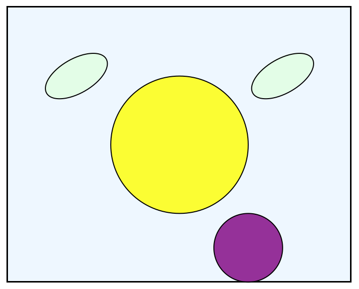
Here is the 2D visualization of a plant cell:
The cell membrane is defined as a rectangle with corners at (0,0) and (10,8), outlined in black, filled with light blue, and set to 50% opacity. The nucleus is represented by a yellow disk centered at (5,4) with a radius of 2, outlined in black and set to 80% opacity. Two chloroplasts, resembling green rotated ovals, are positioned at (2,6) and (8,6) and rotated by Pi/6 radians. The vacuole, displayed as a purple disk centered at (7,1) with a radius of 1, is outlined in black and set to 80% opacity.
In[]:=
Graphics[{EdgeForm[Black],Opacity[0.5],LightBlue,Rectangle[{0,0},{10,8}],EdgeForm[Black],Opacity[0.8],Yellow,Disk[{5,4},2],EdgeForm[Black],Opacity[0.8],LightGreen,Rotate[Disk[{2,6},{1,0.5}],Pi/6],EdgeForm[Black],Opacity[0.8],LightGreen,Rotate[Disk[{8,6},{1,0.5}],Pi/6],EdgeForm[Black],Opacity[0.8],Purple,Disk[{7,1},1]}]
Out[]=
Here is a proportional 3D visualization using the same parameters:
In[]:=
Graphics3D[{Opacity[0.5],LightBlue,Cuboid[{0,0,0},{10,8,2}],Opacity[0.8],Yellow,Sphere[{5,4,1},1.5],Opacity[0.8],LightGreen,Ellipsoid[{2,6,1},{1,0.5,0.5}],Opacity[0.8],LightGreen,Ellipsoid[{8,6,1},{1,0.5,0.5}],Opacity[0.8],Purple,Sphere[{7,1,0.5},1]},Boxed->False]
Out[]=

Light Reaction and Calvin Cycle
Light Reaction and Calvin Cycle
The process of photosynthesis includes two cycles that work in different regions of the chloroplasts within plant cells. The light reaction captures and converts light energy into chemical energy stored in ATP (adenosine triphosphate) and NADPH, which are then used in the Calvin cycle to produce glucose and other organic compounds from carbon dioxide.
First, we represent the light reaction, which takes place in the thylakoid membrane, creating a function called ‘lightReaction’ with the parameters x and y - it takes in the products of light energy and water to output the amount of ATP, NADPH, and oxygen are produced.
We set the initial level of ADP and NADP to 1, and since ATP is directly proportional to light energy and NADPH is proportional to twice the amount of lightEnergy, we can simply calculate the ATP and NADPH production levels with our variables. Next, we can calculate the oxygen levels. One molecule of O2 is produced for every 2 molecules of H2O consumed. The function returns the results as a list of ATP, NADPH, and Oxygen.
In[]:=
lightReaction[x_,y_]:=Module{lightEnergy,water,ADP,NADP,ATP,NADPH,oxygen},lightEnergy=x; water=y;ADP=1;NADP=1;ATP=lightEnergy;NADPH=2*lightEnergy;oxygen=water2;{ATP,NADPH,oxygen}
Here is an example of the lightReaction in use.
In[]:=
lightReaction[20,90]
Out[]=
{20,40,45}
The Calvin cycle, also known as the light-independent reaction, takes place in the stroma of the chloroplasts. It operates independently of light but depends on some of the products generated by the light-dependent reactions during photosynthesis.
This function takes in the products of ATP and NADPH to output the glucose, ATP, and NADPH levels produced. The carbon dioxide level is also a set arbitrary value. Based on the availability of ATP and NADPH, we use the relationship between glucose and the products to yield the smallest value of the three parameters. Then, we update ATP and NADPH levels based on glucose production. The results are a list of glucose, ATP, and NADPH.
This function takes in the products of ATP and NADPH to output the glucose, ATP, and NADPH levels produced. The carbon dioxide level is also a set arbitrary value. Based on the availability of ATP and NADPH, we use the relationship between glucose and the products to yield the smallest value of the three parameters. Then, we update ATP and NADPH levels based on glucose production. The results are a list of glucose, ATP, and NADPH.
In[]:=
calvinCycle[x_,y_]:=Module[{carbonDioxide,ATP,NADPH,glucose},carbonDioxide=x;ATP=y;NADPH=2*y;glucose=Min[carbonDioxide,ATP,NADPH/6];ATP-=glucose;NADPH-=6*glucose;{glucose,ATP,NADPH}]
Here is an example of the calvinCycle function in use:
In[]:=
calvinCycle[15,30]
Out[]=
{10,20,0}
After representing these two crucial cycles as separate functions with arbitrary values, we can utilize them more accurately by applying the observations from global light and water production levels in the Macro section of this project.
How Light Intensity and Temperature Affects ATP and Oxygen Production Levels: A Numerical Representation
How Light Intensity and Temperature Affects ATP and Oxygen Production Levels: A Numerical Representation
ATP Production Levels
ATP Production Levels
This ATP model takes three input parameters—light intensity, temperature, and CO2 concentration—adjusted through sliders (lightSlider, tempSlider, and co2Slider). The Manipulate function updates the ATP level, computed as the product of these parameters, and displays the results in a column format. The sliders have predefined ranges (0 to 100 for light intensity, 0 to 50 for temperature, and 0 to 0.1 for CO2 concentration). We used this to explore the influence of each factor on ATP production in real-time, observing how changes in light intensity, temperature, and CO2 concentration affected the overall simulated photosynthetic process.
In[]:=
Manipulate[Module[{lightIntensity,temperature,co2Concentration,atpLevel},(*photosynthesisATPlevelmodel*)lightIntensity=lightSlider;temperature=tempSlider;co2Concentration=co2Slider;atpLevel=lightIntensity*temperature*co2Concentration;(*Displaytheresult*)Column[{Row[{"Light Intensity: ",lightIntensity}],Row[{"Temperature: ",temperature}],Row[{"CO2 Concentration: ",co2Concentration}],Row[{"ATP Level: ",atpLevel}]}]],(*Controls*){{lightSlider,50,"Light Intensity"},0,100},{{tempSlider,25,"Temperature"},0,50},{{co2Slider,0.04,"CO2 Concentration"},0,0.1},SaveDefinitions->True]
Out[]=


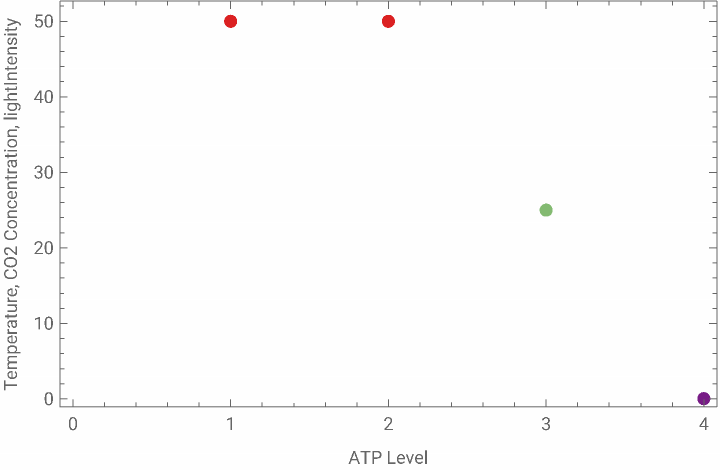
To visualize the wide range of data, colors in the created scatter plot are determined by the option ColorFunction -> “Rainbow” in the ListPlot function. The “Rainbow” color function assigns different colors to data points based on their position along a gradient of colors, ranging from violet to red. In this case, the colors in the scatter plot represent the range of ATP levels. Data points with lower ATP levels are assigned colors from the violet end of the spectrum, while data points with higher ATP levels are assigned colors from the red end. The color provides a visual indication of the magnitude of the ATP level associated with each set of input parameters (light intensity, temperature, and CO2 concentration).
In[]:=
Manipulate[Module[{lightIntensity,temperature,co2Concentration,atpLevel},lightIntensity=lightSlider;temperature=tempSlider;co2Concentration=co2Slider;atpLevel=lightIntensity*temperature*co2Concentration;(*Displaytheresult*)ListPlot[{{atpLevel,lightIntensity,temperature,co2Concentration}},PlotStyle->PointSize[0.02],ColorFunction->"Rainbow",PlotLegends->{"ATP Level"},Frame->True,FrameLabel->{"ATP Level","Temperature, CO2 Concentration, lightIntensity"}]],(*Controls*){{lightSlider,50,"Light Intensity"},0,100},{{tempSlider,25,"Temperature"},0,50},{{co2Slider,0.04,"CO2 Concentration"},0,0.1},SaveDefinitions->True]
Out[]=
Oxygen Production Levels
Oxygen Production Levels
The oxygen model simulates hypothetical photosynthesis oxygen production based on light intensity, temperature, and CO2 concentration. Just like the ATP model, the Manipulate function enables us to dynamically modify the input parameters through sliders and observe the resulting oxygen production. The displayed output consists of numeric values for light intensity, temperature, CO2 concentration, and oxygen production presented in a column format. The sliders for this model also have the same predefined ranges.
To visualize our data from the active sliders, the same process was applied from the ATP model to the oxygen model. The x-axis represents oxygen production, and the y-axis shows a combination of light intensity, temperature, and CO2 concentration.
It is very important to note that for both of these models, the y-axis represents a combination of the three input parameters, where each data point is associated with a unique combination of light intensity, temperature, and CO2 concentration.
We saw that light intensity and CO2 concentration affect the level of ATP in photosynthesis the most. We then saw that temperature affects oxygen production levels the most, while using CO2 and light intensity as constant variables. The finding that temperature has a more substantial influence on oxygen production suggests a greater sensitivity of this process to temperature variations, contributing to our understanding of how different environmental factors may selectively regulate ATP synthesis and oxygen production in a simplified photosynthesis model. Further investigation of this will be seen using data sets of plants in different environments on a macro-level scale.
We saw that light intensity and CO2 concentration affect the level of ATP in photosynthesis the most. We then saw that temperature affects oxygen production levels the most, while using CO2 and light intensity as constant variables. The finding that temperature has a more substantial influence on oxygen production suggests a greater sensitivity of this process to temperature variations, contributing to our understanding of how different environmental factors may selectively regulate ATP synthesis and oxygen production in a simplified photosynthesis model. Further investigation of this will be seen using data sets of plants in different environments on a macro-level scale.
Molecule Visualization
Molecule Visualization
For a more specific, chemical point-of-view of photosynthesis enhancement without the consideration of temperature, we also started with the basic chemical equation of photosynthesis, where we displayed the reactants (water and carbon dioxide) and the products (glucose and oxygen gas).
Chemical Reaction function used
Checking if the reaction is balanced
To visualize all the molecules involved in this reaction, we utilized the various molecular plotting functions.
A molecule of water in 3D
A molecule of carbon dioxide in 3D
A molecule of glucose in 3D
A molecule of oxygen gas in 3D
To now simulate this basic photosynthesis reaction, we developed a function that calculates the number of products in mols given a certain number of reactants in mols. With this simulation, we only looked at a whole number of mols for each molecule.
Since for every 6 carbon dioxide and 6 water molecules, only one molecule of glucose is produced, creating this function to generate the maximum number of glucose molecules produced.
Now using the previous function to return a pair of numbers, the first being the number of glucose molecules produced and the second the number of oxygen molecules
Making a manipulate function to dynamically see how many glucose molecules can be produced
To make a graph of the number of each product based on the initial number of water and carbon dioxide molecules, we looped our function through to get 30 data points and graphed them.
Since there are 30 data points:
Creating the graph for the number of glucose molecules produced
Creating the graph for the number of oxygen molecules produced
Aligning with the first section of the project, this visualization also shows that there is an increase in the amount of oxygen gas produced with the increase of water and carbon dioxide molecules. We see a similar pattern with the production of glucose molecules based on water and carbon dioxide.
Macro-Level Visualization: Photosynthesis Enhancement Across Different Global Data Sets
Macro-Level Visualization: Photosynthesis Enhancement Across Different Global Data Sets
Getting the Data
Getting the Data
The dataset stems from a study (Ellsworth D.S et al.) that aimed to investigate the influence of phosphorus (P) limitations on photosynthesis in tropical and subtropical forests—crucial contributors to carbon isolation. In this study, researchers investigated the crucial role of phosphorus (P) limitations in carbon (C) uptake by tropical forests, which are major contributors to atmospheric carbon sequestration through photosynthesis.
The relationship between photosynthesis and phosphorus concentration in leaves was found to be generally consistent across tropical forests on four continents. The study employed the ORCHIDEE-CNP model and revealed that when phosphorus constraints were implemented, gross photosynthesis decreased by 36% in tropical and subtropical regions compared to traditional nitrogen constraints and unlimited leaf phosphorus. The findings offer a quantitative understanding of the phosphorus dependence of photosynthesis, providing valuable insights for improving global terrestrial carbon models.
We used the dataset obtained from the referenced study, focusing specifically on measurements of photosynthesis rate, carbon dioxide concentration (CO2S), water concentration (H2OS), water conductance (Cond), air temperature (Tair), and nitrogen concentration (Perc_N). The analysis centers on understanding how different parameters influence the photosynthetic activity across diverse leaf samples representing various species
Photosynthesis VS Different Conditions for Various Species
Photosynthesis VS Different Conditions for Various Species
In order to investigate the impact of various parameters on the rate of photosynthesis, our experimental approach involved creating graphical representations. We made graphs where the photosynthesis rate served as the variable on the y-axis, while different parameters were represented on the x-axis. These graphical representations serve as visual tools to elucidate the relationships and trends between photosynthesis and the selected parameters.
The numerical labels in our dataset correspond to distinct leaf samples for each species, and it’s important to note that approximately 10 experiments were conducted for each leaf sample.
The numerical labels in our dataset correspond to distinct leaf samples for each species, and it’s important to note that approximately 10 experiments were conducted for each leaf sample.
Upon analyzing the generated graphs, a noteworthy trend emerges in the relationship between carbon dioxide (CO2) concentration and photosynthesis rate . The observed pattern indicates a relatively linear correlation, where an increase in CO2 concentration is associated with a higher photosynthesis rate . This linearized relationship suggests a positive influence of elevated CO2 levels on photosynthetic activity across the diverse leaf samples studied. Additionally, it is interesting to note that the concentration of nitrogen appears to be the same for each leaf sample, forming a straight line in the graphs depicting this parameter, suggesting a consistent nitrogen concentration across the samples.
In contrast, when exploring the graphs depicting other parameters, a distinct pattern emerges. The graphs for these parameters exhibit a hook-shaped curve, indicative of a more nuanced relationship.
In contrast, when exploring the graphs depicting other parameters, a distinct pattern emerges. The graphs for these parameters exhibit a hook-shaped curve, indicative of a more nuanced relationship.
Following the absence of clear patterns in the relationship between photosynthesis rate and parameters such as water concentration, water conductance, and air temperature, our investigation took a different direction . We were curious whether these parameters were influenced by variations in carbon dioxide (CO2) concentration . To explore this potential dependency, we made graphs with CO2 concentration on the x - axis and water concentration, water conductance, and air temperature on the y - axis . Despite this additional analysis, no discernible correlation was observed between CO2 concentration and these parameters .
Statistics of Photosynthesis Rates
Statistics of Photosynthesis Rates
We found it interesting to explore the statistics of photosynthesis rates . Calculating the average rates for each species and creating a graph based on these averages revealed three outliers in the dataset.
Recognizing the potential influence of outliers on our data distribution, we made the decision to remove some of these atypical points. Subsequently, we employed the “Find Distribution” function to identify and characterize the underlying distribution model of the refined dataset.
The appeal of the Gamma distribution lies in its adaptability to positively skewed datasets, making it particularly suitable for our analysis.
Beyond our research on photosynthesis rates, the Gamma distribution is utilized in diverse fields - it has proven valuable in physics, engineering, finance, biology, and environmental sciences. The ubiquity of the Gamma distribution across multiple areas of research adds an additional layer of interest to its selection as the distributional model for our dataset, showing its relevance in capturing the complexities of real-world phenomena.
Beyond our research on photosynthesis rates, the Gamma distribution is utilized in diverse fields - it has proven valuable in physics, engineering, finance, biology, and environmental sciences. The ubiquity of the Gamma distribution across multiple areas of research adds an additional layer of interest to its selection as the distributional model for our dataset, showing its relevance in capturing the complexities of real-world phenomena.
Statistics of Photosynthesis vs CO2 Concentration
Statistics of Photosynthesis vs CO2 Concentration
In our exploration of the statistical relationship between photosynthesis rates and CO2 concentration, we made a plot featuring the average photosynthesis rates for various plant species against their corresponding CO2 concentrations . Notably, a discernible pattern emerged, with the majority of data points concentrated within the range of 600 to 800 μmol CO2 mol^- 1.
The identification of this concentration range enhances our understanding between photosynthesis rates and CO2 concentration, with valuable insights into the conditions that influence optimal photosynthetic activity across different plant species. Further analysis within this concentration range may reveal nuanced trends and help elucidate the underlying mechanisms governing the observed patterns.
The identification of this concentration range enhances our understanding between photosynthesis rates and CO2 concentration, with valuable insights into the conditions that influence optimal photosynthetic activity across different plant species. Further analysis within this concentration range may reveal nuanced trends and help elucidate the underlying mechanisms governing the observed patterns.
Continental Statistics
Continental Statistics
The data collection for various plant species spanned diverse continents, including Australia, Africa, South America, and Asia. Notably, the distribution of photosynthesis rates exhibited variations across these continents, underscoring the potential influence of regional factors on the observed patterns. Interestingly, despite the differences in distribution, the medians for photosynthesis rates appeared to be relatively similar across all continents.
However, a noteworthy observation emerged when considering outliers within the dataset—they were predominantly from Africa. This intriguing phenomenon suggests that, within the context of this study, Africa may exhibit unique characteristics or environmental conditions that contribute to the presence of atypical data points. Exploring the specific factors contributing to these outliers in the African dataset could provide valuable insights into the regional dynamics influencing photosynthesis rates.
However, a noteworthy observation emerged when considering outliers within the dataset—they were predominantly from Africa. This intriguing phenomenon suggests that, within the context of this study, Africa may exhibit unique characteristics or environmental conditions that contribute to the presence of atypical data points. Exploring the specific factors contributing to these outliers in the African dataset could provide valuable insights into the regional dynamics influencing photosynthesis rates.
Visualising Photosynthesis on Maps
Visualising Photosynthesis on Maps
The next representation of the dataset would be a map representing the continents that include the data, using the same dataset as before. The goal of the last part of macro was to create map visualisation to compare what factors (such as weather and climate, mountains, oceans, and different types of terrains in South America, Australia, Asia, and Africa) to see what qualities benefited growth rates.
Analyzing The Dataset
Analyzing The Dataset
The dataset only includes sites from continents that start with the letter A, South America, Australia, Asia, and Africa. Antarctica is not included because it it likely difficult to collect data from a continent with such cold climates. It is possible to plot all the sites on the map but an easier approach would be to represent the sites by separating the dataset by each continent.
Separating South America
Separating South America
Separating Africa
Separating Africa
Separating Australia
Separating Australia
Separating Asia
Separating Asia
Testing Which Site Names Worked
Testing Which Site Names Worked
Now, in order to plot the sites of where the data was collected, we must extract all the site names from the dataset containing all four continents. The next step would be to test each site in natural language to see if Wolfram recognizes it. The site names don’t necessarily mean that there is more photosynthesis in the areas where sitenames are more common. Instead, the dataset could have just included those specific sites likely due to convenience or preference.
Knowing that there is a possibility that not all site names will work in natural language, we will only use the ones that worked. To compare for later, we know that their were 44 total sites collected.
We used Wolfram’s natural language input to find the locations of the sites. Many of the site names were computable in their original format, but there were also several sites, an example being Davis Creek, where natural language could only recognize it in a different country or, not at all. We checked through the dataset to see which continents these types of sites came from researched them on the internet to see if they existed. Many of the sites were difficult to locate or didn’t have an Entity associated with them, so for the purposes of creating accurate maps, we did not include these.
So, comparing the total amount of site names to the ones that worked, natural language could only recognize about less than half of them. After that, I labeled the site names that worked and separated them by continent.
Here’s a list made to organize the sites. We found that many of the sites from South America came from Peru, and the typical weather is includes humid summers and cloudy, cold winters and this could possibly show that plants grow better in those weathers.
South America:
adelaide riv: perana brazil
Tambopata: PERU
Jenaro Herrera: PERU
Cusco: PERU
Kosnipata: Cuzco, PERU
Manaus: Brazil
San Lorenzo: Argentina
San Pedro: Chile
Australia:
Howard spring: northern territory
Boulia Qld: Queensland
Daly River
Tumbarumba
Asia:
Kratie (Kracheh): city in Cambodia
Kampong Thom: Cambodia
Africa:
Bissiga: Bouglou Faso
Dano: Ioba Burkina Faso
Boabeng, Ngamiland Botswana
Hombori: Mali
Mban Djerem
Plotting the Four Continents on a Map
Plotting the Four Continents on a Map
Regarding the list above, we put each of the sites into the correct continent categories and grouped entities into lists.
South America Map:
Australia Map:
Asia Map:
Africa Map:
Overall, the maps came out decent and served the purpose of representing sites.
With the maps completed to visualize, it is now easier to compare the similarities in each continent. There are many differences in each of the four continents. The reason for the photosynthesis rates in each pf the continents could be connected to the effects of the qualities in each of the continents. Asia is known to be hot, humid, and have very dry winters while Australia is one of the driest continents with occasional rain in the winter. South America’s weather is also known to be very hot and humid with high rainfall, and Africa to have high temperatures throughout the year with little rainfall. Connecting the maps back to our micro-scale analysis, we can see that plants grow reasonably well in hot and humid climates. Paying attention to the qualities in where plants are found could help increase the effectiveness of growth rates as we know where to seed the plants.
Conclusion
Conclusion
From both micro-level and macro-level representations of different aspects of photosynthesis, we found that the rise of temperature plays one of the most significant external roles for the enhancement of this process. A rise in temperature will result in higher levels of oxygen production, a byproduct that will - through the cycle of organism respiration - increase levels of CO2 which will then increase photosynthesis. This trend is also evident in the datasets, where patterns emerge in various hot and tropical regions worldwide, including Africa, indicating a higher frequency of plant data. Yet, on a global-scale view, these discrepancies in plant production/higher photosynthesis levels may be negligible. It is important to acknowledge that from our research, while temperature and CO2 concentration rates can be said to play the most external important roles in influencing photosynthesis in computational models, the overall macro-scale impact may be subject to various factors and complexities that warrant further investigation. We were impressed by the precision with how the photosynthesis data were collected, enabling us to assess the global impact of plant production and taking into account factors such as climate and region.
Citations
Citations
◼
Ellsworth, D.S., Crous, K.Y., De Kauwe, M.G. et al. Convergence in phosphorus constraints to photosynthesis in forests around the world. Nat Commun 13, 5005 (2022). https://doi.org/10.1038/s41467-022-32545-0. https://rdcu.be/dtQj9
◼
Alberts B, Johnson A, Lewis J, et al. Molecular Biology of the Cell. 4th edition. New York: Garland Science; 2002. Chloroplasts and Photosynthesis. Available from: https://www.ncbi.nlm.nih.gov/books/NBK26819/
◼
OpenStax, Concepts of Biology. The Light-Dependent Reactions. OpenStax CNX. May 18, 2016 http://cnx.org/contents/b3c1e1d2-839c-42b0-a314-e119a8aafbdd@9.10
◼
Yang B, Liu J, Ma X, Guo B, Liu B, Wu T, Jiang Y, Chen F. Genetic engineering of the Calvin cycle toward enhanced photosynthetic CO2 fixation in microalgae. Biotechnol Biofuels. 2017 Oct 5;10:229. doi: 10.1186/s13068-017-0916-8. PMID: 29034004; PMCID: PMC5629779.
CITE THIS NOTEBOOK
CITE THIS NOTEBOOK
Enhancing Photosynthesis: Computational Visualizations Through Micro and Macro Scales
by Wolfram Emerging Leaders Program
Wolfram Community, STAFF PICKS, January 2, 2024
https://community.wolfram.com/groups/-/m/t/3094660
by Wolfram Emerging Leaders Program
Wolfram Community, STAFF PICKS, January 2, 2024
https://community.wolfram.com/groups/-/m/t/3094660