On a Pythagorean n-body example
J. M., 1/8/2021
J. M., 1/8/2021
This is an adaptation of an example due to Nick Trefethen, which he ascribes to the Oxford astrophysicist James Binney. In brief, we consider three planets arranged at the corners of a 3-4-5 right triangle interacting according to an inverse-square force law.
We can use the built-in function NBodySimulation to study this example. (In the past, we would need to explicitly set up the ODEs before invoking NDSolve.) Let us integrate up to time :
t=100
dat1=NBodySimulation["InverseSquare",{<|"Mass"1,"Position"{0,0},"Velocity"{0,0}|>,<|"Mass"1,"Position"{3,0},"Velocity"{0,0}|>,<|"Mass"1,"Position"{0,4},"Velocity"{0,0}|>},100];
To set the mood, let us generate a “starry” background:
bg=BlockRandom[SeedRandom[42];Graphics[{Directive[GrayLevel[0.9,0.8],AbsolutePointSize[1]],Point[RescalingTransform[{{0,1},{0,1}},{{-8,6},{-2,6}}][RandomReal[1,{150,2}]]]},BackgroundBlack,PlotRange{{-8,6},{-2,6}}]]
We can now visualize the simulation:
Manipulate[Show[bg,Graphics[MapIndexed[{Directive[ColorData[97]@@#2,AbsolutePointSize[8]],Point[#1]}&,dat1[All,"Position",t]]]],{t,0,100},SaveDefinitionsTrue]
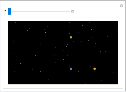
Trefethen notes that the system is supposed to be “self-ionizing”, where one planet goes off in one direction and the other two go off as a pair in the opposite direction. But, we do not observe this in the simulation above!
One thing to try is to change the integration method. LSODA is used by default, but there are other algorithms available. Let’s try using implicit Runge-Kutta:
dat2=NBodySimulation["InverseSquare",{<|"Mass"1,"Position"{0,0},"Velocity"{0,0}|>,<|"Mass"1,"Position"{3,0},"Velocity"{0,0}|>,<|"Mass"1,"Position"{0,4},"Velocity"{0,0}|>},100,Method"ImplicitRungeKutta"];
Visualize the result:
Manipulate[Show[bg,Graphics[MapIndexed[{Directive[ColorData[97]@@#2,AbsolutePointSize[8]],Point[#1]}&,dat2[All,"Position",t]]]],{t,0,100},SaveDefinitionsTrue]
Finally!
Note that the first simulation gave no warnings at all, so this is a reminder that it is often useful to check results of a numerical method, even when there is no immediate indication of error. In practice, one would try not only implicit Runge-Kutta, but other methods that are appropriate.
Now, apart from trying other methods, one can also do a check by evaluating at arbitrary precision. Whenever this is feasible, it is an excellent verification method.
dat1hi=NBodySimulation["InverseSquare",{<|"Mass"1,"Position"{0,0},"Velocity"{0,0}|>,<|"Mass"1,"Position"{3,0},"Velocity"{0,0}|>,<|"Mass"1,"Position"{0,4},"Velocity"{0,0}|>},100,WorkingPrecision20];
Manipulate[Show[bg,Graphics[MapIndexed[{Directive[ColorData[97]@@#2,AbsolutePointSize[8]],Point[#1]}&,dat1hi[All,"Position",t]]]],{t,0,100},SaveDefinitionsTrue]
For completeness, let us both use higher precision, and change the method used for integrating the ODEs. This time, we use the method, which is appropriate for high-precision evaluations:
dat2hi=NBodySimulation["InverseSquare",{<|"Mass"1,"Position"{0,0},"Velocity"{0,0}|>,<|"Mass"1,"Position"{3,0},"Velocity"{0,0}|>,<|"Mass"1,"Position"{0,4},"Velocity"{0,0}|>},100,Method"StiffnessSwitching",WorkingPrecision20];
Manipulate[Show[bg,Graphics[MapIndexed[{Directive[ColorData[97]@@#2,AbsolutePointSize[8]],Point[#1]}&,dat2hi[All,"Position",t]]]],{t,0,100},SaveDefinitionsTrue]