There was an error in the original post. The FinancialDerivative[] function can be used with NonlinearModelFit if the inputs parameters have _?NumericQ. On the post I divided days by 365, because that was needed for Black-Scholes, but not the Mathematica function.
In[]:=
amcall=americanCall[k,days,intrate,σ,div,curprice]
Out[]=
americanCall[k,162,0.0425,σ,0.007908,758.725]
In[]:=
nlm1=NonlinearModelFit[callPrices,amcall,{{σ,0.3}},k]nlm1["BestFitParameters"]

Out[]=
FittedModel
Out[]=
{σ0.364905}
In[]:=
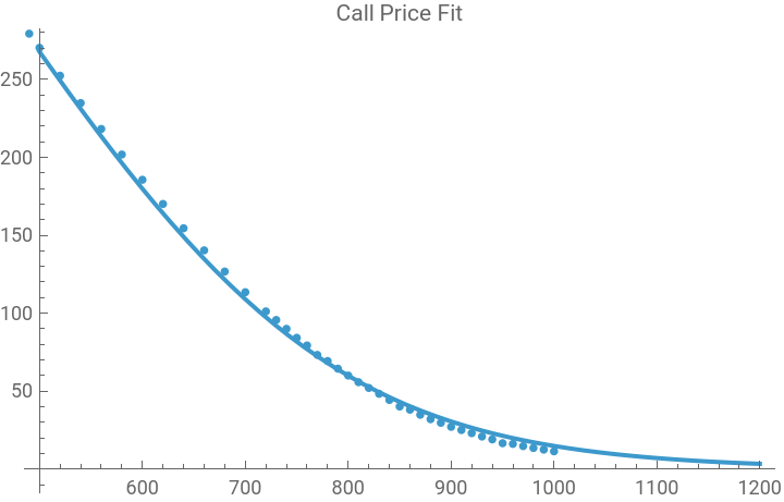
Plot[amcall/.nlm1["BestFitParameters"],{k,500,1200},PlotLabel->"Call Price Fit"];Show[%,ListPlot[callPrices]]
Out[]=
In[]:=
volam=σ/.nlm1["BestFitParameters"]
Out[]=
0.364905
In[]:=
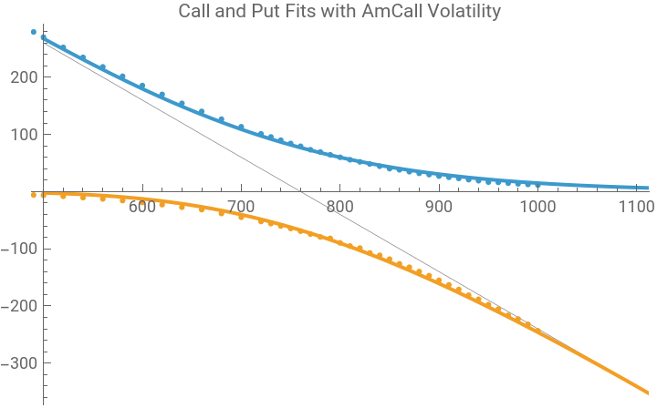
g4=Plot[{americanCall[k,days,intrate,volam,div,curprice],-americanPut[k,days,intrate,volam,div,curprice]},{k,500,1200}];Show[g0,g1,g4,PlotLabel->"Call and Put Fits with AmCall Volatility"]
Out[]=