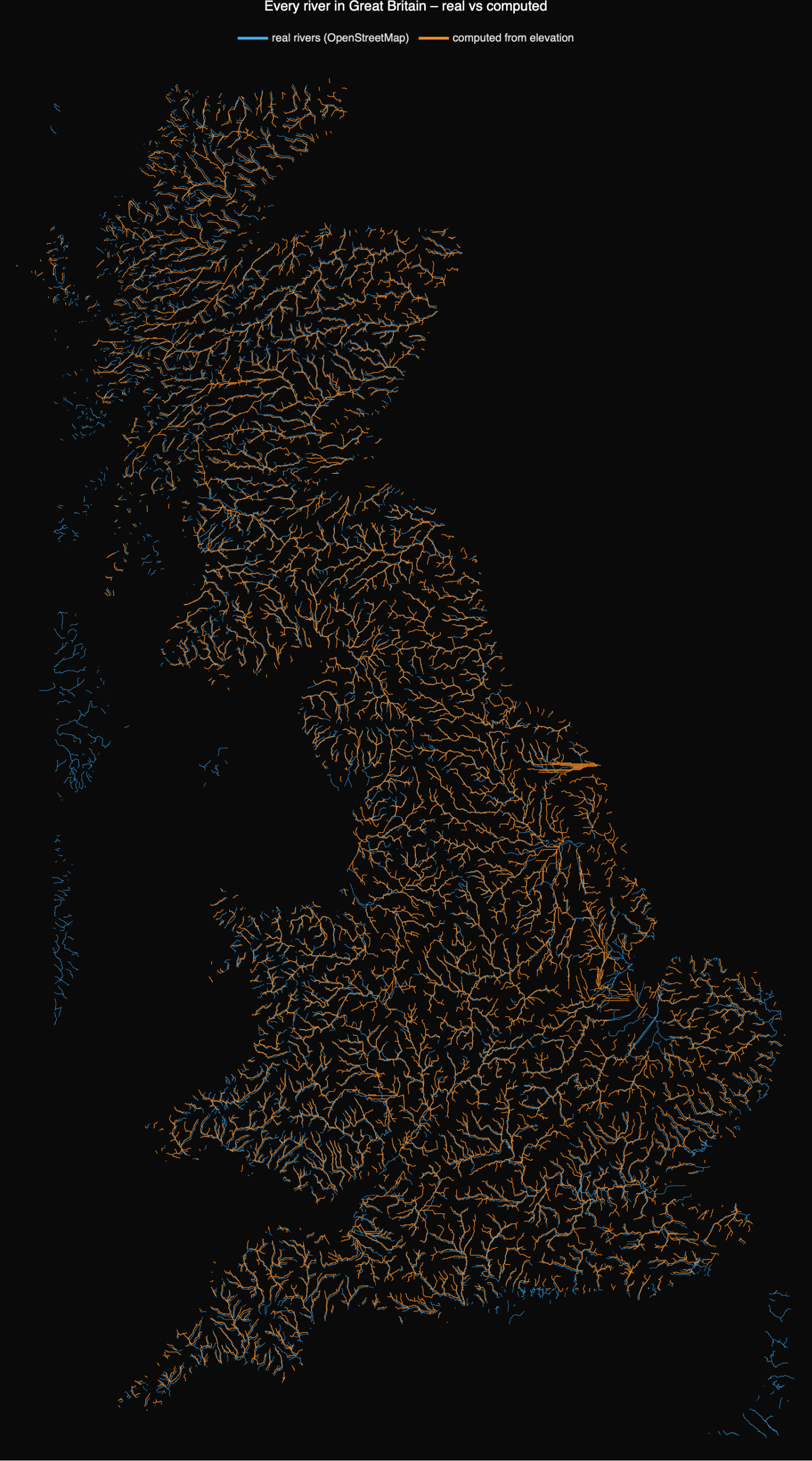
The drainage networks our pipeline computes from bare elevation, laid over the real rivers of OpenStreetMap
In the companion post we took a Digital Elevation Model – nothing but a grid of land-surface heights – filled its pits, routed the flow downhill, and watched a river network fall out of the arithmetic. The natural question is: are those computed rivers the *real* rivers? The model never saw a map. It knows only elevation. So this notebook puts the two side by side: in blue, every real river of Great Britain as mapped by OpenStreetMap; in orange, every channel our pipeline computed from the elevation model. Where they coincide, physics has rediscovered geography.
The answer, visible above, is that they overlap almost everywhere – the orange computed network traces the blue real one across the whole island. That is a genuine validation: starting from heights alone, with no hydrographic data whatsoever, the steepest-descent flow routing reconstructs the actual drainage of Britain. The disagreements are informative too, and we come to them at the end.
1. Setup: the computed rivers
1. Setup: the computed rivers
Load the package and build the computed networks. The Great Britain forest is the same multi-outlet extraction as in the main post (a single ~500 m DEM, 2.9 million cells); the Dee and the Don are the two Aberdeenshire catchments. Each is a one-line call that downloads its own terrain from the built-in GeoElevationData and runs the full fill → flow → accumulate → network pipeline. We wrap each in rnxGeoreference, which corrects one subtlety that matters the moment you overlay on a real map: GeoElevationData returns a grid snapped outward to its tile pyramid, covering a slightly larger area than the bounding box you asked for, so the raw lat/lon labels (and cell sizes) are off. rnxGeoreference recovers the true bounds by correlating the terrain against elevation sampled at known coordinates.
SetDirectory[NotebookDirectory[]];
Get["RiverNetworkX.wl"];
gb = rnxGeoreference @ rnxBuildGreatBritain[]; (* ~6 min, multi-outlet forest of mainland Britain *)
dee = rnxGeoreference @ rnxBuildCatchment["Dee"];
don = rnxGeoreference @ rnxBuildCatchment["Don"];
Get["RiverNetworkX.wl"];
gb = rnxGeoreference @ rnxBuildGreatBritain[]; (* ~6 min, multi-outlet forest of mainland Britain *)
dee = rnxGeoreference @ rnxBuildCatchment["Dee"];
don = rnxGeoreference @ rnxBuildCatchment["Don"];
2. The real rivers, from OpenStreetMap
2. The real rivers, from OpenStreetMap
For ground truth we need real river courses as lines. Wolfram's built-in River entities carry a river's source and mouth but not its full course, so we go to OpenStreetMap, the open crowd-sourced map of the world, and ask its Overpass API for every way tagged waterway=river inside a bounding box. The helper rnxFetchOSMRivers wraps that query and returns a list of {lat, lon} polylines. (waterway=river is the named-river network – streams, canals and ditches are tagged separately – which is the right counterpart to the trunk channels our pipeline extracts.)
osmGB = rnxFetchOSMRivers[{{49.9, 58.7}, {-6.3, 1.8}}]; (* ~30,000 real river ways *)
Length[osmGB]
Length[osmGB]
That single call returns about 30,000 river segments (roughly 1.5 million vertices) for mainland Britain – the real hydrographic network, drawn and checked by tens of thousands of mappers on the ground.
3. Overlay: computed vs real, all of Britain
3. Overlay: computed vs real, all of Britain
Now draw both on the same map: real rivers in blue, computed rivers in orange. rnxFigRealVsComputed handles the projection (an equal-area planar projection about the central latitude) and the styling. This is the headline image at the top of the post.
rnxFigRealVsComputed[osmGB, {gb},
"Title" -> "Every river in Great Britain – real vs computed",
"ImageSize" -> {880, 1520}]
"Title" -> "Every river in Great Britain – real vs computed",
"ImageSize" -> {880, 1520}]
The two networks are nearly coincident from Cornwall to Sutherland – the Severn, Thames, Trent, Great Ouse, Tay, Spey and Clyde systems are all reconstructed in the right places, with the right branching. Remember that the orange lines were produced with no map at all: only the shape of the land and the rule that water runs downhill.
4. A closer look: the Dee and the Don
4. A closer look: the Dee and the Don
Zooming in to the two Aberdeenshire rivers shows the agreement in detail. The orange computed channels of the Dee (south) and the Don (north) thread straight down the blue valleys of the real rivers; the extra blue lines around them are the neighbouring catchments we did not extract here.
osmDD = rnxFetchOSMRivers[{{56.78, 57.50}, {-3.95, -2.00}}];
rnxFigRealVsComputed[osmDD, {dee, don},
"Title" -> "The Dee and the Don – real (OSM) vs computed from elevation",
"ImageSize" -> {1150, 740}]
rnxFigRealVsComputed[osmDD, {dee, don},
"Title" -> "The Dee and the Don – real (OSM) vs computed from elevation",
"ImageSize" -> {1150, 740}]
5. How well do they agree – and where they don't
5. How well do they agree – and where they don't
What matches. The trunks and major tributaries line up almost everywhere: the large-scale drainage of Britain is set by topography, and steepest-descent routing on a decent DEM recovers it faithfully. This is the reassuring result – and a reminder that a drainage map is, to first order, a derivative of the elevation surface.
◼
Resolution. The Great Britain network is computed on a coarse ~500 m grid, so the orange channels are blockier than the finely-surveyed OSM lines, and the very smallest tributaries are missing. A finer DEM (as in the bare-earth Dee of the main post) closes that gap.
◼
Definition. "waterway=river" in OSM and "accumulation above a threshold" in our pipeline are not the same cut: OSM excludes streams and ditches, while our threshold may include some, so the orange network is sometimes denser in the headwaters and the blue denser in mapped lowland drains.
◼
Estuaries and flats. Where the land is nearly flat – the Fens, tidal estuaries, the Somerset Levels – flow direction is ambiguous and the computed channels can wander or run along the coast, the one place the overlay visibly parts. Real rivers there are partly artificial (embanked, pumped, canalised), which no purely physical model can know.
The honest summary: from elevation alone, the pipeline reconstructs the real river network of an entire country to a striking degree – strong evidence that the geometry of rivers really is governed by the physics of water on a landscape, exactly the premise the Horton–Strahler statistics in the main post rest on. The places it fails are the places where human engineering, not topography, now decides where the water goes.
Data & reproducing it
Data & reproducing it
This notebook is self-contained: evaluate it and it rebuilds the computed networks from the built-in GeoElevationData and re-fetches the real rivers live from OpenStreetMap. The only files needed beside it are RiverNetworkX.wl (the pipeline + rnxFetchOSMRivers + rnxFigRealVsComputed) and an internet connection for the Overpass query.
Real rivers: © OpenStreetMap contributors, made available under the Open Database License (ODbL) – www.openstreetmap.org/copyright, via the Overpass API. Computed rivers and elevation: Wolfram GeoElevationData. Code MIT, text & figures CC-BY-4.0. Companion to "River networks from elevation data – Horton–Strahler statistics of the Dee and the Don."