ABSTRACT (original article): We provide an in silico study of stochastic viral infection extinction from a pharmacokinetical viewpoint. Our work considers a non-specific antiviral drug that increases the virus clearance rate, and we investigate the effect of this drug on early infection extinction. Infection extinction data are generated by a hybrid multiscale framework that applies both continuous and discrete mathematical approaches. The central result of our paper is the observation, analysis and explanation of a linear relationship between the virus clearance rate and the probability of early infection extinction. The derivation behind this simple relationship is given by merging different mathematical toolboxes. CITATION (original article): N. Juhász, F. A. Bartha, S. Marzban, R. Han and G. Röst, Probability of early infection extinction depends linearly on the virus clearance rate, R. Soc. Open Sci. 11: 240903. https://doi.org/10.1098/rsos.240903
This is the Wolfram Mathematica notebook for our article https://royalsocietypublishing.org/doi/full/10.1098/rsos.240903
In[]:=
theoreticalColor="TropicalRainForest";experimentalColor="Bittersweet";lineFitColor="Razzmatazz";histogramColor="Asparagus";zeroFreqColor="Razzmatazz";zeroFreqColorAtF="ShamRock";
In[]:=
vrrrangemax=19.58537402425683`;lineStyle={Thickness[0.005],ColorData["Crayola"]["Purple"],Dashed};lineK=Line[{{vrrrangemax,0},{vrrrangemax,1.1}}];
Experimental probability of extinction values
Experimental probability of extinction values
The values below are calculated via our hybrid system available on GitHub, see https://github.com/msjuhasznora/linearity
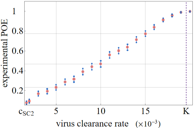
Each element in the list below represents a (c, PoE) pair, where PoE stands for Probability of Extinction.
Each element in the list below represents a (c, PoE) pair, where PoE stands for Probability of Extinction.
In[]:=
experimentalList={{1.67,78/1000},{2,95/1000},{3,169/1000},{4,193/1000},{5,233/1000},{6,288/1000},{7,315/1000},{8,391/1000},{9,441/1000},{10,469/1000},{11,559/1000},{12,602/1000},{13,637/1000},{14,714/1000},{15,774/1000},{16,839/1000},{17,912/1000},{18,957/1000},{19,989/1000},{20,997/1000}};experimentalListForErrorPlot={{1.67,78/1000},{2,95/1000},{3,169/1000},{4,193/1000},{5,233/1000},{6,288/1000},{7,315/1000},{8,391/1000},{9,441/1000},{10,469/1000},{12,602/1000},{13,637/1000},{15,774/1000},{16,839/1000},{17,912/1000},{18,957/1000},{19,989/1000}};experimentalListFunc=Interpolation[experimentalList];
We calculate confidence intervals for these PoE values, see:
https://en.wikipedia.org/wiki/Binomial_proportion_confidence_interval
https://en.wikipedia.org/wiki/Binomial_proportion_confidence_interval
In[]:=
experimentalList95CIUpper=experimentalList;experimentalList95CILower=experimentalList;
In[]:=
For[i=1,i<=Length[experimentalList],i++,experimentalList95CIUpper[[i]][[2]]=experimentalList[[i]][[2]]+1.96*Sqrt[experimentalList[[i]][[2]]*(1-experimentalList[[i]][[2]])]/Sqrt[1000]]
In[]:=
For[i=1,i<=Length[experimentalList],i++,experimentalList95CILower[[i]][[2]]=experimentalList[[i]][[2]]-1.96*Sqrt[experimentalList[[i]][[2]]*(1-experimentalList[[i]][[2]])]/Sqrt[1000]]
In[]:=
ExperimentalCIEndPoints=ListPlot[{experimentalList95CILower,experimentalList95CIUpper},PlotStyle->{{ColorData["Crayola"]["Denim"],PointSize[0.008]},{ColorData["Crayola"]["Denim"],PointSize[0.008]}}];
In[]:=
ExperimentalCILines=Table[Graphics[{ColorData["Crayola"]["Denim"],Line[{{experimentalList95CILower[[n,1]],experimentalList95CILower[[n,2]]},{experimentalList95CIUpper[[n,1]],experimentalList95CIUpper[[n,2]]}}]}],{n,1,Length[experimentalList]}];
In[]:=
p1=ListPlot{experimentalList},PlotStyle{{ColorData["Crayola"][experimentalColor],PointSize[0.015]}},FrameLabel{Row[{"virus clearance rate (",Style["×",26],")"}],"experimental POE"},PlotTheme->"Scientific",LabelStyle->Directive[FontFamily->"Times",Black,FontSize->30],PlotRange{{1.44,20.3},{0.055,1.1}},TicksStyle->Medium,GridLines->{{0,5,10,15},Map[experimentalListFunc[#]&,{5,10,15}]},FrameTicks->{{{{0,"0 "},0.2,0.4,0.6,0.8,{1,"1 "}},None},{{{1.67,Subscript["c","SC2"]},5,10,15,{vrrrangemax,"K"}},None}},Epilog->{Directive[lineStyle],lineK},ImageSizeScaled[0.4];
-3
10
In[]:=
Show[p1,ExperimentalCIEndPoints,ExperimentalCILines]
Best linear fit to observed PoE values
Best linear fit to observed PoE values
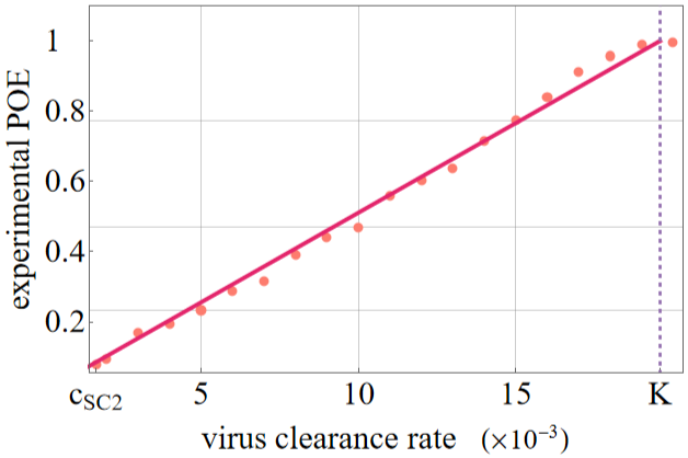
We calculate the best linear fit to our data and determine the value to measure goodness of fit.
2
R
In[]:=
lineFit=Fit[experimentalList,{x},x]
Out[]=
0.0510585x
In[]:=
myLinearFunction[x_]:=0.05105850921006065`x
In[]:=
avg=N[Sum[experimentalList[[i]][[2]],{i,1,Length[experimentalList]}]/Length[experimentalList]]
Out[]=
0.5326
In[]:=
1-Sum[(experimentalList[[i]][[2]]-myLinearFunction[experimentalList[[i]][[1]]])^2,{i,1,Length[experimentalList]}]/Sum[(experimentalList[[i]][[2]]-avg)^2,{i,1,Length[experimentalList]}]
Out[]=
0.993862
As expected, goodness of fit is suitable.
In[]:=
p2=Show[p1,Plot[lineFit,{x,1.44,vrrrangemax},PlotStyle->{ColorData["Crayola"][lineFitColor],Thickness[0.007]}]]
In[]:=
Solve[lineFit==1,x]
Out[]=
{{x19.5854}}
Note: towards the end (when c is close to K), the end of the straight line seems mollified -- in this region E(X) >>1 does not really hold.
Comparing experimental PoE values with 1/R0
Comparing experimental PoE values with 1/
R
0
Here we compare our experimental Probability of Extinction values with our experimental 1/ values. All data points come from our hybrid model referenced above.
R
0
In[]:=
oneOverExperimentalR0={{1.67,1/12.456},{2,1/9.938},{3,1/6.775},{4,1/4.971},{5,1/4.076},{6,1/3.562},{7,1/2.738},{8,1/2.609},{9,1/2.143},{10,1/2.08},{11,1/1.957},{12,1/1.587},{13,1/1.546},{14,1/1.446},{15,1/1.253},{16,1/1.236},{17,1/1.167},{18,1/1.098},{19,1/1.055}};
In[]:=
ExperimentalR0={{1.67,12.456},{2,9.938},{3,6.775},{4,4.971},{5,4.076},{6,3.562},{7,2.738},{8,2.609},{9,2.143},{10,2.08},{11,1.957},{12,1.587},{13,1.546},{14,1.446},{15,1.253},{16,1.236},{17,1.167},{18,1.098},{19,1.055}};
In[]:=
R0STD={{1.67,Sqrt[163.28]},{2,Sqrt[96.30]},{3,Sqrt[50.84]},{4,Sqrt[34.428]},{5,Sqrt[22.828]},{6,Sqrt[15.074]},{7,Sqrt[10.827]},{8,Sqrt[8.252]},{9,Sqrt[6.266]},{10,Sqrt[6.2]},{11,Sqrt[5.529]},{12,Sqrt[3.8444]},{13,Sqrt[3.535]},{14,Sqrt[3.3]},{15,Sqrt[2.61]},{16,Sqrt[2.676]},{17,Sqrt[2.215]},{18,Sqrt[2.118]},{19,Sqrt[2.1199]}};
In[]:=
R0List95CIUpper=ExperimentalR0;R0List95CILower=ExperimentalR0;
In[]:=
For[i=1,i<=Length[ExperimentalR0],i++,R0List95CIUpper[[i]][[2]]=(ExperimentalR0[[i]][[2]]+1.96*R0STD[[i]][[2]]/Sqrt[1000])]
In[]:=
For[i=1,i<=Length[ExperimentalR0],i++,R0List95CILower[[i]][[2]]=(ExperimentalR0[[i]][[2]]-1.96*R0STD[[i]][[2]]/Sqrt[1000])]
In[]:=
oneOverR0List95CIUpper=oneOverExperimentalR0;oneOverR0List95CILower=oneOverExperimentalR0;
In[]:=
For[i=1,i<=Length[oneOverExperimentalR0],i++,oneOverR0List95CIUpper[[i]][[2]]=1/R0List95CILower[[i]][[2]]]
In[]:=
For[i=1,i<=Length[oneOverExperimentalR0],i++,oneOverR0List95CILower[[i]][[2]]=1/R0List95CIUpper[[i]][[2]]]
In[]:=
oneOverR0CIEndPoints=ListPlot[{oneOverR0List95CILower,oneOverR0List95CIUpper},PlotStyle->{{ColorData["Crayola"]["Denim"],PointSize[0.008]},{ColorData["Crayola"]["Denim"],PointSize[0.008]}},PlotMarkers->Graphics[{Rectangle[]},ImageSize->3]];
In[]:=
oneOverR0CILines=Table[Graphics[{ColorData["Crayola"]["Denim"],Line[{{oneOverR0List95CILower[[n,1]],oneOverR0List95CILower[[n,2]]},{oneOverR0List95CIUpper[[n,1]],oneOverR0List95CIUpper[[n,2]]}}]}],{n,1,Length[oneOverExperimentalR0]}];
In[]:=
lineFit1OverR0=Fit[oneOverExperimentalR0,{x},x]
Out[]=
0.0502809x
Determining the offspring distribution
Determining the offspring distribution
Virus removal rate \in [1.67 , 18] * E-3
Virus removal rate \in [1.67 , 18] * E-3
We use this data to determine the offspring distribution.
How many times do we have 0 offspring, how many times we have 1, hoe many times we have 2, etc (out of 1000 simulations):
check if the expected value is > 1 (it is a condition in the fix point theorem)
Observation: we seem to have a reasonable fit to geometric distribution. This holds for a wide range of c values (virus clearance rate).
For completeness we consider the distribution fit tests below.
The test for geometric distribution verifies our hypothesis.
The distribution in question is clearly not a Poisson distribution.
The test for negative binomial distribution is considered for completeness. The first parameter is close to 1, the second parameter is close to the parameter of the geometric distribution. This, again, corresponds to our expectations.
Testing various distributions.
Testing various distributions.
The Maximum Likelihood estimate of the geometric distribution’s parameter.
The Maximum Likelihood estimate of the geometric distribution’s parameter.
In this chapter we visualize the geometric distribution’s parameter as a function of c.
This looks similar to part of the 1/(1+(a/x)^n) curve. The underlying function might be described by a Hill equation with n=1.
Confidence intervals
Confidence intervals
We calculate 95% confidence intervals for the data points.
95% CI with a Bootstrap approach:
95% CI with a Bootstrap approach:
Fisher information approach.
Fisher information approach.
Fitted curve
Fitted curve
The fitted curve matches our data points in a suitable manner.
Branching processes: the theoretical PoE
Branching processes: the theoretical PoE
Using the above observation regarding a reasonable fit to geometrical distribution, the PoE is given by the fix point of the PGF of the geometrical distribution.
The POE is given by
G_X(λ)=λ
λ / (1 - (1-λ)x) = x, thus we have
λ = x * (1 - (1-λ)x)
We have a simple second order equation. The non-negative solution to that is:
The POE is given by
G_X(λ)=λ
λ / (1 - (1-λ)x) = x, thus we have
λ = x * (1 - (1-λ)x)
We have a simple second order equation. The non-negative solution to that is:
We have seen that λ = λ(c), where we found that λ = λ(c) takes the following form: λ(c) = 1 / (1 + 19.27/c)
Altogether we have
λ / (1 - (1-λ)POE) = POE and
λ(c) = 1 / (1 + 19.27/c)
λ / (1 - (1-λ)POE) = POE and
λ(c) = 1 / (1 + 19.27/c)
The probability of extinction is given (below on the LHS) as a function of λ, and for that to be a linear function of c we need the following:
Which corresponds to what we have previously observed.
CITE THIS NOTEBOOK
CITE THIS NOTEBOOK
Probability of early infection extinction depends linearly on the virus clearance rate
by Nóra Juhász, Ferenc A. Bartha, Sadegh Marzban, R. Han & G.Röst
Wolfram Community, STAFF PICKS, October 24, 2024
https://community.wolfram.com/groups/-/m/t/3307502
by Nóra Juhász, Ferenc A. Bartha, Sadegh Marzban, R. Han & G.Röst
Wolfram Community, STAFF PICKS, October 24, 2024
https://community.wolfram.com/groups/-/m/t/3307502