In[]:=
Needs["DPLN`"]
Here is my argument that it would be better to place these things into the Mathematica kernel. Maybe your colleagues could help.
The AsymmetricLaplaceDistribution is simply the distribution of the difference of two ExponentialDistribution random variables with different parameters. What Wolfram Language delivers is a mess!
In[]:=
al=TransformedDistribution[x-y,{xExponentialDistribution[α],yExponentialDistribution[β]}]
Out[]=
VarianceGammaDistribution1,,(-α+β),0
α+β
2
1
2
In[]:=
PDF[al,x]
Out[]=
|
In[]:=
Simplify[PDF[al,x],{α>0,β>0}]CharacteristicFunction[al,t]//Simplify
Out[]=
|
Out[]=
αβ
(t+α)(t-β)
In[]:=
PDF[AsymmetricLaplaceDistribution[α,β],x]CharacteristicFunction[AsymmetricLaplaceDistribution[α,β],t]
Out[]=
|
Out[]=
αβ
(t+α)(t-β)
The NormalLaplaceDistribution is the distribution of the sum of random variables from an AsymmetricLaplaceDistribution and a NormalDistribution.
In[]:=
nlp=TransformedDistribution[x-y+z,{xExponentialDistribution[α],yExponentialDistribution[β],zNormalDistribution[μ,σ]}]
Out[]=
TransformedDistributionx.1-x.2+x.3,x.1ExponentialDistribution[α],x.2ExponentialDistribution[β],x.3NormalDistribution[μ,σ]
In[]:=
pdf=PDF[nlp,x];//AbsoluteTimingpdf
Out[]=
{21.3044,Null}
Out[]=
αβα-2x+2μ+αErfc+β2x-2μ+βErfc
1
2
2
σ
-x+μ+α
2
σ
2
σ1
2
2
σ
x-μ+β
2
σ
2
σ2(α+β)
In[]:=
PDF[NLDistribution[α,β,μ,σ],x]
Out[]=
αβErfc+Erfc
α-x+μ+
α
2
σ
2
-x+μ+α
2
σ
2
σβx-μ+
β
2
σ
2
x-μ+β
2
σ
2
σ2(α+β)
In[]:=
PDF[NLDistribution[α,β,μ,σ],x]==pdf//Simplify
Out[]=
True
In[]:=
cf=CharacteristicFunction[nlp,t];//AbsoluteTimingcf
Out[]=
{0.0138741,Null}
Out[]=
tμ-
2
t
2
σ
2
(t+α)(t-β)
In[]:=
CharacteristicFunction[NLDistribution[α,β,μ,σ],t]
Out[]=
tμ-
2
t
2
σ
2
(t+α)(t-β)
The DPLNDistribution is the distribution of the exponentiation of a NormalLaplaceDistribution random variable.
In[]:=
dpln=TransformedDistribution[Exp[x-y+z],{xExponentialDistribution[α],yExponentialDistribution[β],zNormalDistribution[μ,σ]}]
Out[]=
TransformedDistribution,x.1ExponentialDistribution[α],x.2ExponentialDistribution[β],x.3NormalDistribution[μ,σ]
x.1-x.2+x.3
In[]:=
pdfe=PDF[dpln,x];//AbsoluteTimingpdfe
Out[]=
$Aborted
Out[]=
pdfe
These take forever.
In[]:=
Plot[PDF[dpln/.{α->3,β->4,μ->0,σ->1},x],{x,-3,3},PlotRange->All]//AbsoluteTiming
Out[]=
$Aborted
In[]:=
PDF[DPLNDistribution[α,β,μ,σ],x]
Out[]=
αβErfc+Erfc
αμ+-Log[x]
α
2
σ
2
μ+α-Log[x]
2
σ
2
σβ-μ++Log[x]
β
2
σ
2
-μ+β+Log[x]
2
σ
2
σ2x(α+β)
In[]:=
Plot[PDF[DPLNDistribution[3,4,0,1],x],{x,0,3},PlotRange->All]
Out[]=
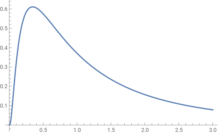
These distributions if implemented in the kernel would just fall off the tree with TransformedDistribution[]. In the current kernel the DPLN is practically impossible, even though they are related to relatively simple distributions conceptually when you think about sums and exponentiation of random variables. They are in the literature. https://www.math.uvic.ca/faculty/reed/