Overview
Overview
This notebook studies the classic consecutive-parallel reaction network A → P → S, A → S (e.g., partial oxidation of benzene, A, to the desired intermediate maleic anhydride, P, which can further over-oxidize to combustion products, S). Because P is an unstable intermediate, there is a genuine trade-off between converting more of the feed A and preserving the P already formed. The notebook computes the reactor's attainable region in the (CA, CP) plane, extracts the Pareto-efficient (non-dominated) frontier of that trade-off, and finds the economically optimal operating point for three feedstock-price scenarios using a weighted-sum (tangent-line) argument.
In[]:=
v0=0.0025;cA0=10;
Setup. v0 is the reactor's volumetric flow rate and cA0 is the feed concentration of A. These set the scale for the mole balances solved below.
In[]:=
rateConstants[T_]:={4280Exp[-12660/T],(*k1*)70100Exp[-15000/T],(*k2*)26Exp[-10800/T](*k3*)};
Kinetics. rateConstants[T] returns Arrhenius-type rate constants k1 (A->P), k2 (P->S), and k3 (A->S) as functions of absolute temperature T, using pre-exponential factors 4280, 70100, 26 and activation-energy/R terms 12660, 15000, 10800.
Solve the PFR ODEs for a given T, return sampled {cA,cP} pairs over W
trajectory[T_,Wmax_:10000,n_:600]:=Module[{k1,k2,k3,sol,Wgrid},{k1,k2,k3}=rateConstants[T];sol=NDSolve[{v0cA'[W]==-(k1+k3)cA[W],cA[0]==cA0,v0cP'[W]==k1cA[W]-k2cP[W],cP[0]==0},{cA,cP},{W,0,Wmax}][[1]];Wgrid=Subdivide[0.,Wmax,n];{Wgrid,{cA[#],cP[#]}&/@Wgrid/.sol}];
Reactor model. trajectory[T, Wmax, n] integrates the packed-bed (plug-flow) mole balances for A and P as functions of catalyst weight W:
v0 dCA/dW = -(k1+k3) CA
and
v0 dCP/dW = k1 CA - k2 CP,
with CA(0)=cA0 and CP(0)=0.
NDSolve integrates this ODE system numerically, and the result is sampled at n+1 evenly spaced points from W=0 to W=Wmax. data600 evaluates this trajectory at T=600 (the reactor temperature).
v0 dCA/dW = -(k1+k3) CA
and
v0 dCP/dW = k1 CA - k2 CP,
with CA(0)=cA0 and CP(0)=0.
NDSolve integrates this ODE system numerically, and the result is sampled at n+1 evenly spaced points from W=0 to W=Wmax. data600 evaluates this trajectory at T=600 (the reactor temperature).
In[]:=
data600=trajectory[600];
Attainable region. pall plots CP/cA0 versus CA/cA0 (normalized by the feed concentration) as W increases: this traces the reachable concentration trajectory - CA falls monotonically as more catalyst is contacted, while CP first rises (net production of P) and then falls once the P->S degradation (k2) dominates.
In[]:=
pall=ListPlotdata600[[2]]10,AspectRatio->1,GridLines->Automatic,Joined->True,PlotStyle->Darker@Red,FrameLabel"[0]","[0]",Frame->True,PlotRange->{{0,1},{0,1}}
C
A
C
A
C
P
C
A
Out[]=
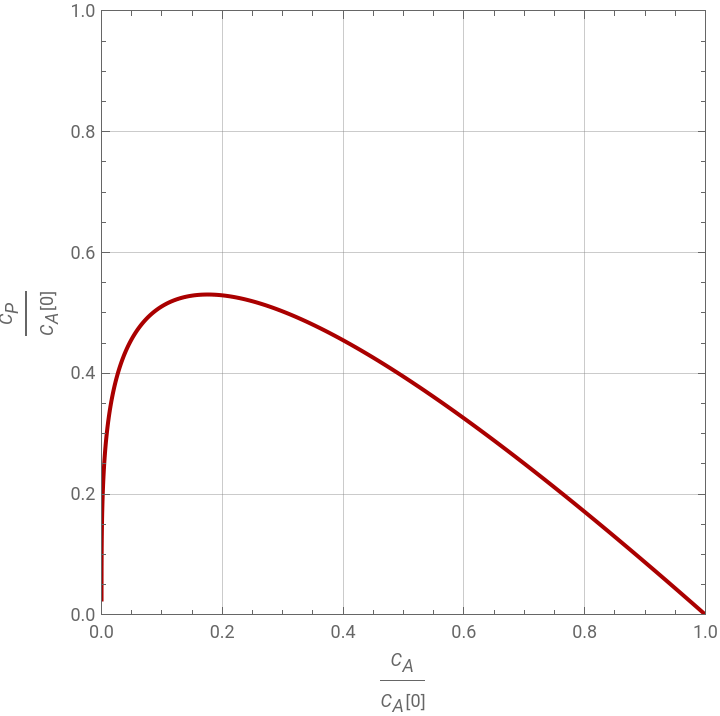
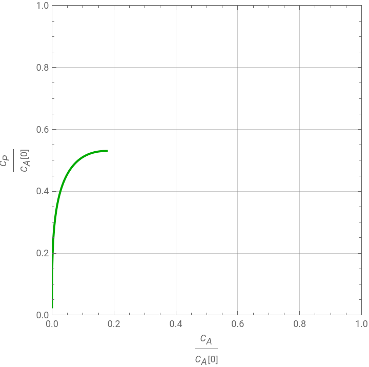
Pareto filter. paretoFilter performs a standard non-dominated sort for two objectives (minimize CA, maximize CP): sort the points by CA ascending, then keep only the points whose CP is a new running maximum. This trims the trajectory to the efficient branch, discarding everything past the CP peak, since those points are dominated - equal or lower CP could be had with less catalyst (i.e., more A remaining, or lower conversion cost) elsewhere on the curve.
Non-dominated filter: minimize cA, maximize cP. Sort ascending by cA, keep points whose cP is a new running maximum.
paretoFilter[pts_List]:=Module[{sorted,runningMax=-Infinity,keep={}},sorted=SortBy[pts,First];Scan[If[#[[2]]>runningMax,AppendTo[keep,#];runningMax=#[[2]]]&,sorted];keep];
front, frontCA, and frontCP hold the resulting Pareto-efficient points and their coordinates, and pfront plots this frontier (in green) on the same normalized axes.
In[]:=
front=paretoFilter[data600[[2]]/10];frontCA=front[[All,1]];frontCP=front[[All,2]];
In[]:=
pfront=ListPlotfront,AspectRatio->1,GridLines->Automatic,Joined->True,PlotStyle->{Darker@Green},FrameLabel"[0]","[0]",Frame->True,PlotRange->{{0,1},{0,1}}
C
A
C
A
C
P
C
A
Out[]=
Economic overlay. CostA and CostP represent the relative cost of feed A versus the value of product P. ratios defines three price-ratio scenarios (r = CostA/CostP-like quantities): a case where benzene is cheap (r=0.5), the base case (r=CostA/CostP), and a case where benzene is expensive (r=1.4). This ratio expresses how many units of lost feed value are equivalent to one unit of product value.
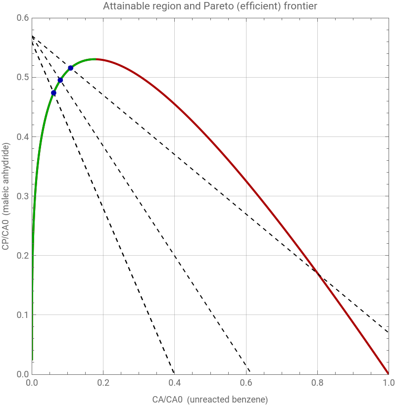
Weighted-sum optimum. For each price ratio r, this forms the linear objective CP - r*CA and finds the frontier point that maximizes it (Ordering[obj, -1] locates the index of the maximum). This is the classic weighted-sum scalarization of a two-objective optimization: geometrically, it is equivalent to sliding a line of slope r along the frontier until it is tangent to it - that tangency point is the profit-maximizing operating point for the given price ratio. optPoints stores {CA*, CP*, r} for each of the three scenarios.
Economic overlay: weighted-sum optimum on the frontier for beta/alpha price ratios
CostA=6;CostP=6.5;(*beta,alpha,basecasefromtheoriginalnotebook*)ratios={"cheap benzene"->0.5,"base case (6/6.5)"->CostA/CostP,"expensive benzene"->1.4};
tangentLines builds the dashed tangent line (slope r) through each optimal point, illustrating the geometric tangency condition described above.
In[]:=
optPoints=Association[Map[Function[rule,Module[{label=rule[[1]],r=rule[[2]],obj,i},obj=frontCP-rfrontCA;i=First@Ordering[obj,-1];label->{frontCA[[i]],frontCP[[i]],r}]],ratios]];
optMarkers places a marker at each of the three optimal (CA*, CP*) points.
In[]:=
tangentLines=KeyValueMap[Function[{label,val},Module[{ca,cp,r,x0,x1},{ca,cp,r}=val;{x0,x1}={0,cA0}/cA0;{Dashed,Line[{{x0,cp-r(x0-ca)},{x1,cp-r(x1-ca)}}]}]],optPoints];
Final figure. This combines the attainable-region trajectory (red), the Pareto frontier (green), the tangent lines (dashed), and the optimal markers (blue) into one annotated plot, "Attainable region and Pareto (efficient) frontier," with axes CA/CA0 (unreacted benzene) and CP/CA0 (maleic anhydride).
In[]:=
optMarkers=KeyValueMap[Function[{label,val},{PointSize[0.015],Point[{val[[1]],val[[2]]}]}],optPoints];
In[]:=
Show[pall,pfront,Graphics[{tangentLines,{Darker@Blue,optMarkers}}],PlotRange->{{0,cA0},{0,6}}/cA0,Frame->True,FrameLabel->{"CA/CA0 (unreacted benzene)","CP/CA0 (maleic anhydride)"},PlotLabel->"Attainable region and Pareto (efficient) frontier",ImageSize->400,GridLines->Automatic]
Out[]=
Results. This prints CA*/cA0 and CP*/cA0 for each of the three price scenarios - the economically optimal stopping point (catalyst weight / conversion level) for cheap, base-case, and expensive benzene.
The profit-optimal point for three price scenario
These results makes physical/economic sense : when benzene (A) is cheap relative to the product (low r), it' s not worth pushing conversion very hard—you stop closer to the point of maximum P yield, leaving more A unreacted . When benzene is expensive (high r), the model pushes toward higher conversion (lower CA*) even though that sacrifices some P yield to secondary degradation, because wasting expensive feedstock costs more than the lost product value .
CITE THIS NOTEBOOK
CITE THIS NOTEBOOK
Pareto analysis of a packed-bed reactor for a consecutive-parallel reaction network
by Housam Binous
Wolfram Community, STAFF PICKS, September 23, 2026
https://community.wolfram.com/t/28149/1
by Housam Binous
Wolfram Community, STAFF PICKS, September 23, 2026
https://community.wolfram.com/t/28149/1