CITE THIS NOTEBOOK: Lagrangian mechanics 2D of rolling body by Emmy Blumenthal. Wolfram Community JAN 31 2023.
Here, we simulate the motion of a 2D convex body rolling on a flat surface by deriving the equation of motion from Lagrangian mechanics.
Introduction
Introduction
Lagrangian mechanics is a method in classical mechanics which provides a systematic process for deriving the equations of motion of a dynamical system that is parameterized by somewhat arbitrary coordinates. An interesting exercise is to derive and solve the equations of motion for the dynamics of an irregularly-shaped body rolling on a flat table. This problem is somewhat challenging because it requires creative procedures to efficiently evaluate quantities necessary to solve the equations of motion in a reasonable amount of time. The results are interesting because the solutions have various, complex behaviors which depend on the shape of the body on the table. Additionally, we can create a satisfying visualization. To begin, I solve a simplified 2D problem; in a future post, I will provide a solution to the 3D problem.
The essential assumption in this problem is that the 2D rolling body is *convex*. This means that the body’s orientation can be specified by the point that is in contact with the table. In order for the body to rest against the flat surface, the normal vector of the edge of the body at the point of contact must be anti-parallel to the normal vector of the flat surface. This means that the only coordinate in this problem will be that which specifies the point of contact. This coordinate will have a countable number of values that specify the same point on the body but distinct points on the flat surface; this specification will account for rolling.
Many technical details and most code will be relegated to the attached notebook.
Defining the convex body
Defining the convex body
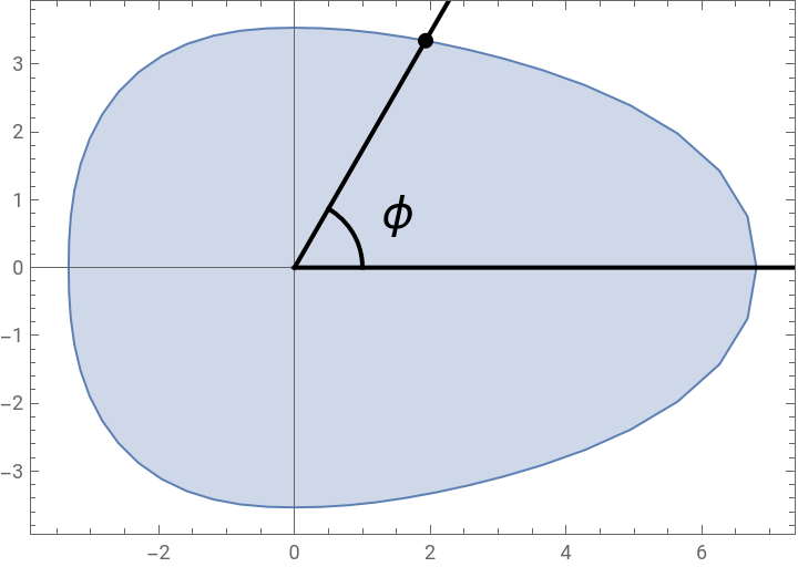
We begin by defining a body to be the interior of the curve in polar coordinates: ; the coordinate will come to specify the point of contact with the surface. Here is a figure of an example body in units of centimeters:
ρ(r)
r_init.(r,ϕ)rρ(ϕ)(cosϕ,sinϕ)
ϕ
In[]:=
(*WeworkinstandardSIunitsWedefinetheconvexbodyinpolarcoordinates:*)rrinit[ϕ_]=0.05;
-4/9
+(1.5+Sin[ϕ-π/2])
9/8
(2)
2
Cos[ϕ-π/2]
9/8
()
2
Sin[ϕ-π/2]
In[]:=
ParametricPlotrrrinit[ϕ]{Cos[ϕ],Sin[ϕ]},{r,0,1},{ϕ,0,2π},Epilog->Thick,HalfLine[{0,0},{1,0}],HalfLine[{0,0},RotationMatrix[π/3].{1,0}],PointSize[Large],Point{rrinit[ϕ]{Cos[ϕ],Sin[ϕ]}}/.ϕ->π3,Circle[{0,0},1,{0,π/3}],Text[Style["",FontSize->20,FontFamily->"CMU Classical Serif"],{1.5,0.8}]
2
10
2
10
ϕ
Out[]=
Density:
In[]:=
ρ[r_,ϕ_]=25.;
In[]:=
UnitConvertQuantityρ[r,ϕ],"Kilograms","Grams"
2
"Meters"
2
"Centimeters"
Out[]=
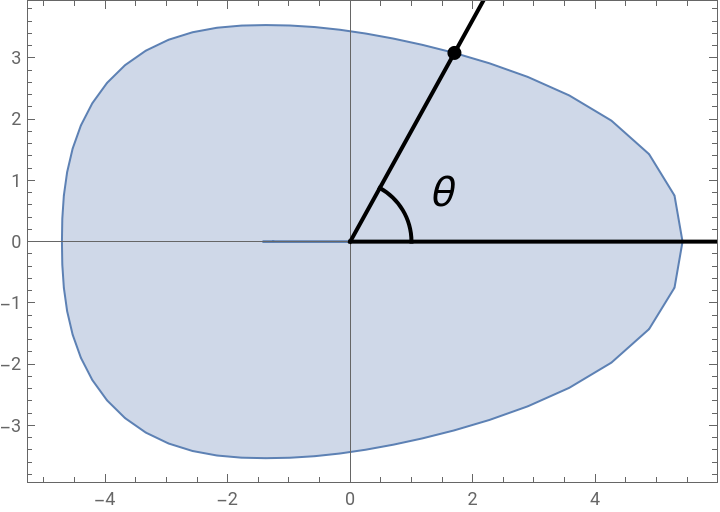
Next, we compute the mass and center of mass of the body:where is the mass of the body, is the density, and is the Jacobian of . For the figure shown above, I chose , so , . Next, we subtract the center of mass so that the body is now defined by the parametric equation . To capture dynamics later, we define an angle such that :
r_com
m∫∫D(r,ϕ)
2π
_0
1
_0
detJ
dϕdrT
J
r_comD(r,ϕ)r_init.(r,ϕ)
1
m
2π
_0
1
_0
detJ
dϕdr,T
J
m
D(r,ϕ)
J
(r,ϕ)↦r_init.(r,ϕ)
D(r,ϕ)2.5
2
g/cm
m143.1 g
r_com(1.379,0)cm
r(r,ϕ)r_init.(r,ϕ)-r_com
θ(ϕ)
tanθ(ϕ)r(r,ϕ))_2/r(r,ϕ))_1
In[]:=
mass=NIntegrateρ[r,ϕ]Evaluate
Det[#.#]
&[D[rrrinit[ϕ]{Cos[ϕ],Sin[ϕ]},{{r,ϕ}}]],{ϕ,0,2π},{r,0,1}Out[]=
0.143089
In[]:=
UnitConvert[Quantity[mass,"Kilograms"],"Grams"]
Out[]=
In[]:=
vol=NIntegrateEvaluate
Det[#.#]
&[D[rrrinit[ϕ]{Cos[ϕ],Sin[ϕ]},{{r,ϕ}}]],{ϕ,0,2π},{r,0,1}Out[]=
0.00572356
In[]:=
UnitConvert[Quantity[vol,],]
2
"Meters"
2
"Centimeters"
Out[]=
In[]:=
relCom=NIntegrateρ[r,ϕ]rrrinit[ϕ]{Cos[ϕ],Sin[ϕ]}Evaluate
1
mass
Det[#.#]
&[D[rrrinit[ϕ]{Cos[ϕ],Sin[ϕ]},{{r,ϕ}}]],{ϕ,0,2π},{r,0,1}//Chop//N//QuietOut[]=
{0.0137868,0.}
In[]:=
UnitConvert[Quantity[relCom,"Meters"],"Centimeters"]
Out[]=
,
Now, we subtract the center of mass:
In[]:=
rr[r_,ϕ_]=rrrinit[ϕ]{Cos[ϕ],Sin[ϕ]}-relCom;
In[]:=
ParametricPlotrr[r,ϕ],{r,0,1},{ϕ,0,2π},Epilog->Thick,HalfLine[{0,0},{1,0}],HalfLine[{0,0},RotationMatrix[ArcTan@@rr[1,π/4]].{1,0}],PointSize[Large],Point{rr[1,ϕ]}/.ϕ->π4,Circle[{0,0},1,{0,ArcTan@@rr[1,π/4]}],Text[Style["",FontSize->20,FontFamily->"CMU Classical Serif"],{1.5,0.8}]
2
10
2
10
θ
Out[]=
Additionally, we will need the moment of inertia:
In[]:=
momI=NIntegrateρ[r,ϕ]rr[r,ϕ].rr[r,ϕ]Evaluate
Det[#.#]
&[D[rr[r,ϕ],{{r,ϕ}}]],{ϕ,0,2π},{r,0,1}Out[]=
0.000141525
In[]:=
UnitConvert[Quantity[momI,"Kilograms"],"Grams"]
2
"Meters"
2
"Centimeters"
Out[]=
Next, we compute the normal vector:
In[]:=
normal[ϕ_]=#
#.#
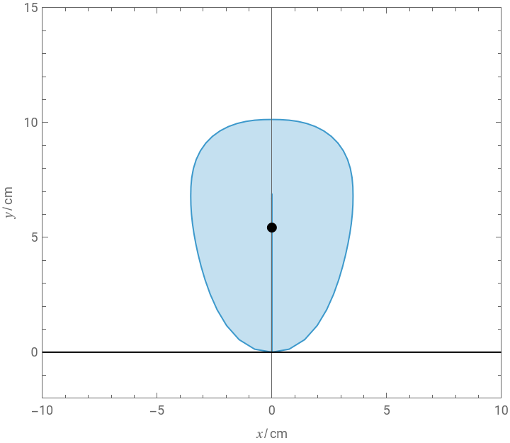
&[RotationMatrix[-π/2].D[rr[r,ϕ],ϕ]/.r->1];Now, we define a matrix that rotates the convex body so that the point on the surface with polar coordinate ϕ rests against the table has a normal vector perpendicular to the table:
In[]:=
rotmat[ϕ_]:=RotationMatrix[{normal[ϕ],{0,-1}}];
In[]:=
ManipulateParametricPlotrotmat[ϕ].rrr.,ϕ.-rr[1,ϕ],r.,0,1,ϕ.,0,2π,Epilog->{InfiniteLine[{0,0},{1,0}],PointSize[Large],Point[-rotmat[ϕ].rr[1,ϕ]]},PlotRange->{{-10,10},{-2,15}},FrameLabel->{"",""},{ϕ,0,2π},SaveDefinitions->True
2
10
2
10
x/cm
y/cm
Out[]=


Now, we want to analyze how the body rolls along the table. To do this, we first define the length traveled when moving to some angle ϕ along the surface of the body
In[]:=
distInit[ϕ_]:=NIntegrate
Drr1,ϕ.,ϕ..Drr1,ϕ.,ϕ.
,ϕ.,0,ϕIn[]:=
dist=Interpolation[Table[{ϕ,distInit[ϕ]},{ϕ,-20π,20π,π/10.}]]
Out[]=
InterpolatingFunction


In[]:=
ManipulateParametricPlotrotmat[ϕ].rrr.,ϕ.-rr[1,ϕ]+{dist[ϕ],0},r.,0,1,ϕ.,0,2π,Epilog->{InfiniteLine[{0,0},{1,0}],PointSize[Large],Point[-rotmat[ϕ].rr[1,ϕ]+{dist[ϕ],0}]},PlotRange->{{-0.6,0.6},{-0.02,0.15}},{ϕ,-3π,3π},SaveDefinitions->True
Out[]=

Next, we define the position of the center of mass as a function of the angular position of the contact point
Let’s plot the center of mass as a function of angle:
Because we shifted the origin and the center of mass and the origin do not explicitly align, the angle to the point of contact relative to the center of mass, θ, is not the same as ϕ. The relation θ(ϕ) can be calculated:
The relationship between $\theta$ and $\phi$ can be found by taking a derivative of the above formula and integrating to yield an increasing function (as opposed to a periodic function). Here is a plot of this relationship:
Defining the Lagrangian and the equations of motion
Defining the Lagrangian and the equations of motion
Because we subtracted the center of mass when defining ${\bf r}$ earlier, the kinetic energy of the rolling body is the sum of rotational and translational kinetic energy:
The equation of motion is given by the Euler–Lagrange equation:
Solving the equations of motion and visualizing the solution
Solving the equations of motion and visualizing the solution
Because the equation of motion does not have an explicit form for the derivative, we need to specify a method to solve for the derivatives during numerical solutions:
The Hamiltonian and phase portrait
The Hamiltonian and phase portrait
We have defined a non-dissipative dynamical system with a Lagrangian, so we can define a Hamiltonian and use it to plot orbits in phase space. The Hamiltonian is given by:
By using ContourPlot, we can create a phase portrait. On this phase portrait, we can also highlight two separatrices which separate two types of librations (inside green and pink curves) and hindered rotations (outside pink curve); this terminology is borrowed from the description of the phase portrait of the plane pendulum dynamical system.