Due to its computational irreducibility, predicting behaviour of cellular automata is a difficult, almost impossible task. However, can we induce the behaviour of a cellular automaton? More specifically, can we control its shape? In order to answer these questions, an experiment was conducted to evolve various cellular automata configurations to a specific shape, considering cellular automata boundary as its fitness function.
Analysing Different Configurations
Analysing Different Configurations
An analysis was conducted on various cellular automata types, varying the number of colors (k) and the neighborhood radius (r). The initial focus was on {k = 2, r = 2} configuration, initially the idea was to consider both symmetric and non-symmetric cases. Although, symmetric rules were ultimately selected as the primary focus due to their superior visualization. The main information is summarized using a density plot, where it’s possible to observe which cells are more common in the rules, along with line plots with the frequency of it’s shapes.
For this configuration, the number of distinct shapes is relatively low: only 60 for symmetric shapes.
Out[]=
k=2, r=2, symmetric |
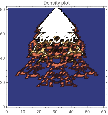

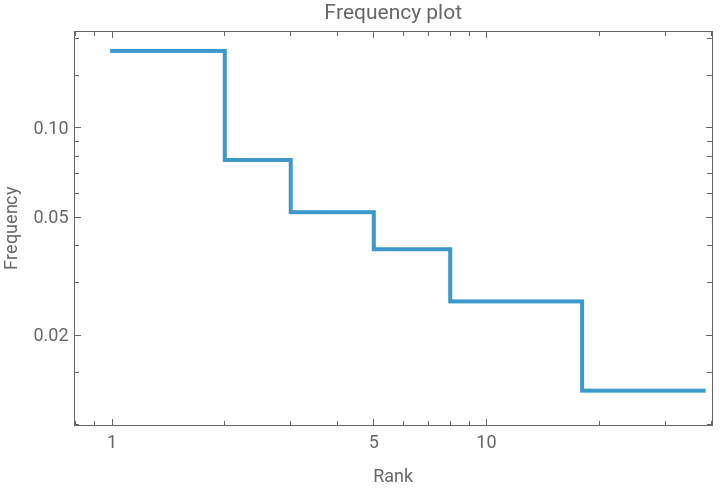
Since the possible shapes are limited with this configuration, and there is a lack of shape variety, configurations with two colors were not used in this evolution process.
For the {k = 3, r = 1} configuration, the number of different shapes are over 7807.
Out[]=
k=3, r=1, symmetric |
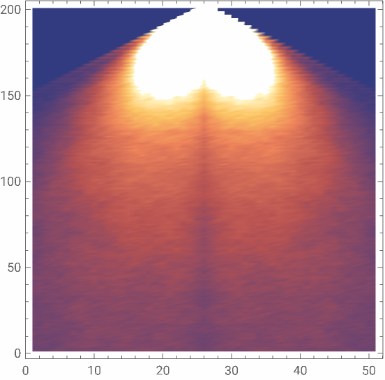
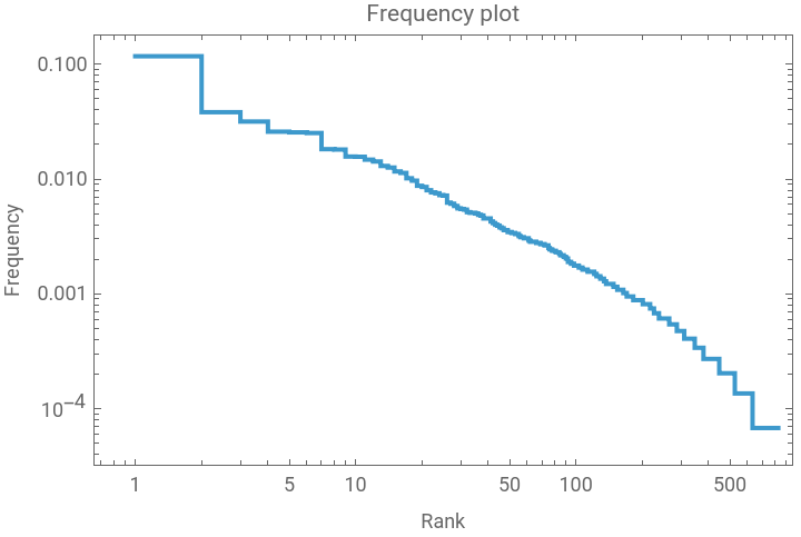
Adapting to Shape
Adapting to Shape
Aiming evolve an automaton toward a specific shape, several formats based on the geometric forms were established, the process to choose these shapes was based on the observation of the most common silhouettes and their geometric representations. Some shapes generated randomly were also tested, sometimes achieving a high fitness level. The success of this process depends of the shape and the number of colors.
Some successful shapes for a lifetime up to 50 steps are:
Out[]=
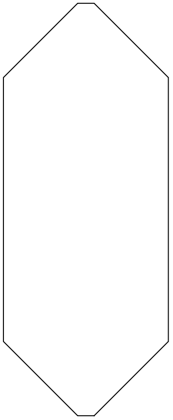

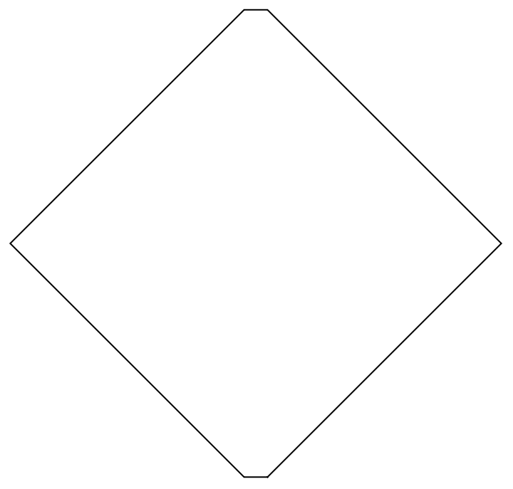
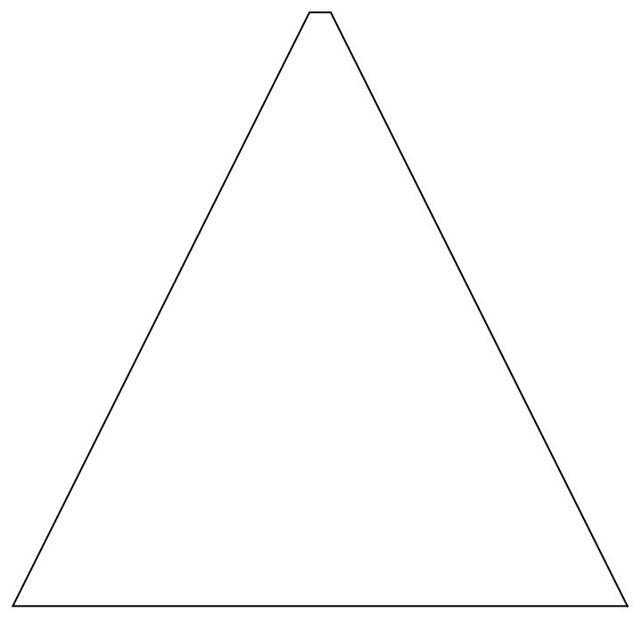
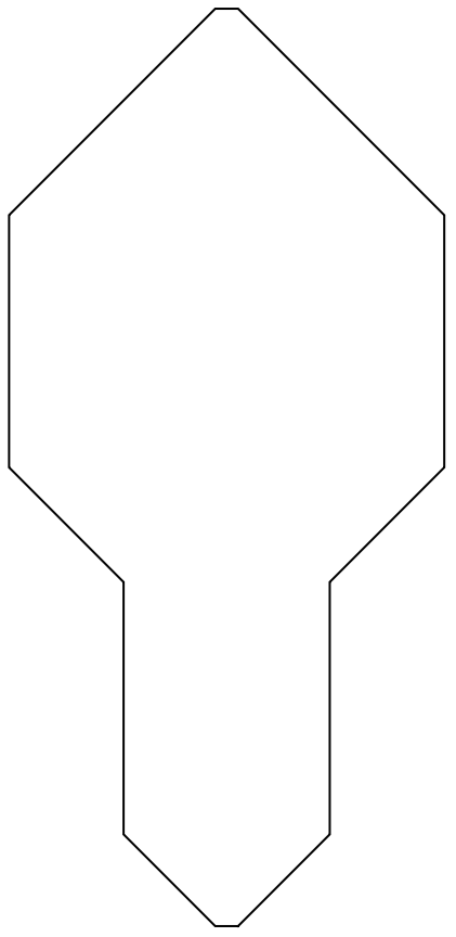
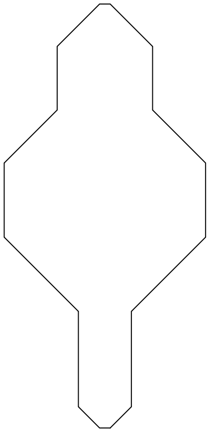
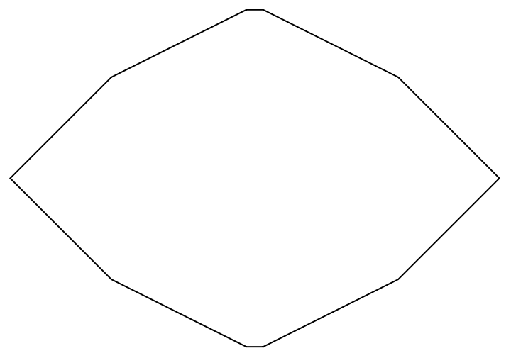
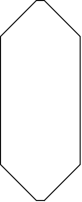
Other shapes were considered, but they had a lower fitness rate, so they were discarded. One of them is displayed bellow.
Out[]=
The evolution of the cellular automata were made using the “AdaptiveCellularAutomaton” function. This function implements a biological evolution algorithm with some parameters to control the evolution process, they include the cellular automaton rule configuration, the mutation rule, the fitness function and the number of mutations made. The parameters used are:
◼
Cellular automata rule configuration: the evolution starts with the cellular automaton rule 0, initialized with a single cell in state 1, surrounded by cells in state 0.
◼
Mutation rule: random mutations are applied at single points within the automaton, with each mutation either maintaining or increasing the fitness value.
◼
Fitness function: the fitness function compares the automaton’s boundary shape to the target shape, calculating the fitness value based on the absolute difference between the two shapes.
◼
Number of mutations: the evolution tries to do 10 000 mutations.
To select the most successful case, the “AdaptiveCellularAutomaton” function was executed multiple times using the “ParallelTable” resource. With these results, it is possible to select the most fit and understand the overall behaviour of the cellular automata configuration in relation to this fitness shape.
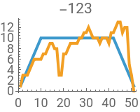
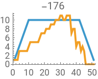
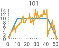
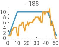
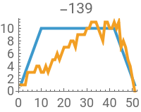
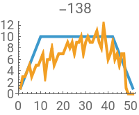
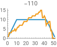
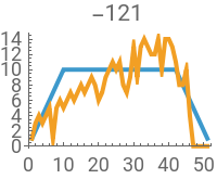
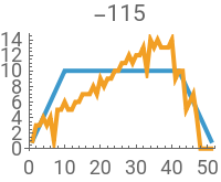
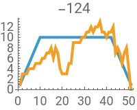
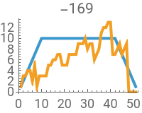
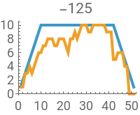
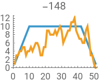
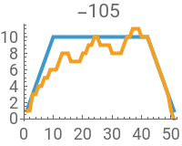
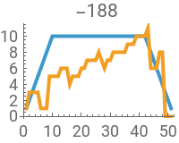
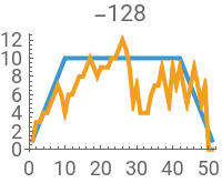
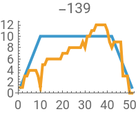
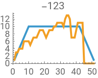
During the investigation, approximately 100 evolutions were analyzed for each shape and number of states. To illustrate this process more clearly, the following 20 graphics presents the results of the evolution for the six-vertex shape.
Out[]=
,
,
,
,
,
,
,
,
,
,
,
,
,
,
,
,
,
,
,
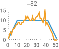
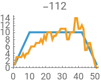
In each plot, the fitness function is shown in blue, and the boundary of the cellular automaton is shown in yellow, with the corresponding fitness value displayed above. Since the primary focus is on symmetric rules, both the fitness function and the boundary are presented as if they were cut in half. This representation makes it easier to visualize the fitness and simplifies the selection of the best cases.
Another way to visualize this data is by plotting the cellular automata achieved in the end of each evolution:
Out[]=
|
|
|
|
|
|
|
|
|
| ||||||||||||||||||||
|
|
|
|
|
|
|
|
|
|




















It is also possible to visualize the evolution breakthroughs (when the mutations lead to a greater fitness value) for each case, following is the evolution of the best case on the simulation sample.
Out[]=
|
|
|
|
|
|
|
|
|
| ||||||||||||||||||||
|
|
|
|
| | | | | |
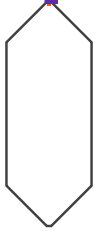
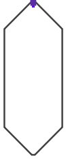













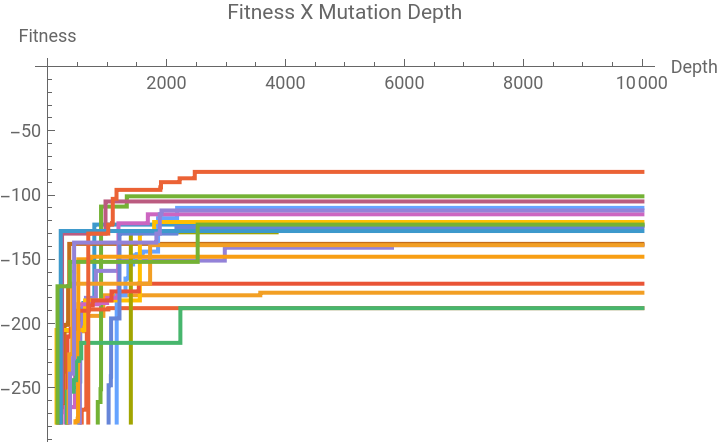
For a more general visualization of the evolution, it is also possible to visualize the fitness value over the mutations:
Out[]=
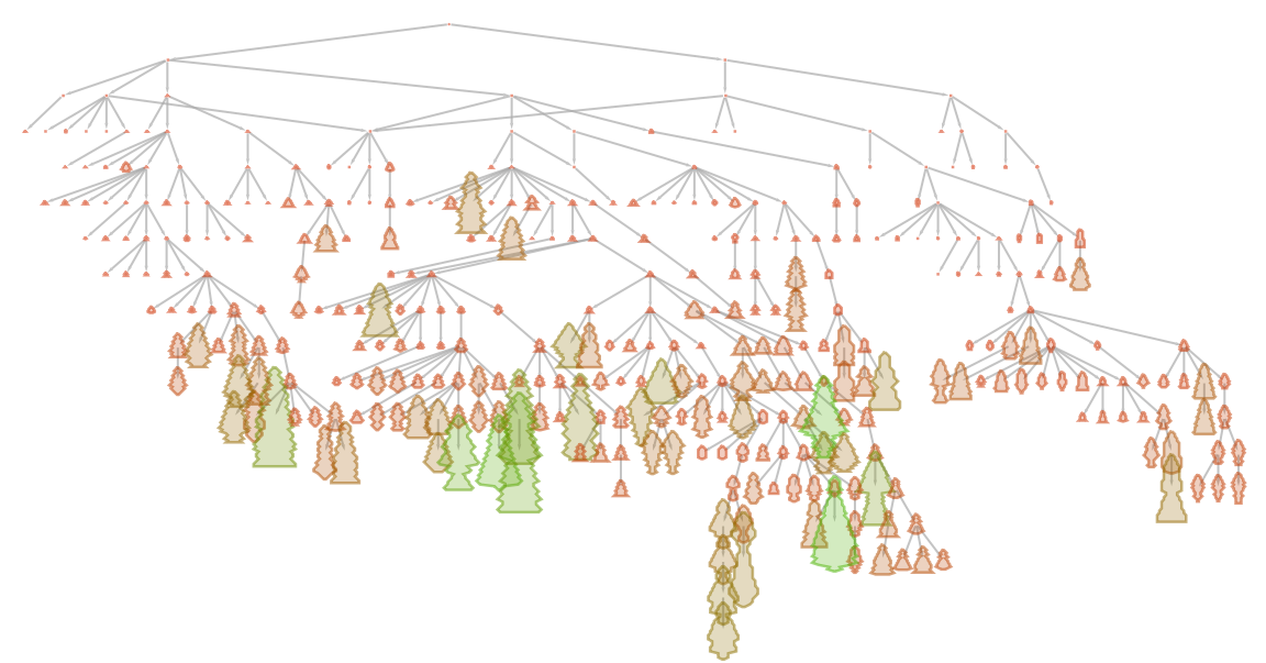
One way to visualize how the “AdaptiveCellularAutomaton” function works is by plotting a graph of its evolution, where each node represents a shape and edges connect shapes that can evolve into one another. The graph below illustrates the evolution of a random case (unrelated to the previous example), where the green nodes represent shapes with higher fitness.
Out[]=
Comparing Results by States
Comparing Results by States
To better understand how the number of states influences the automaton’s ability to evolve toward a specific shape, a comparison was made using the same initial conditions but varying the color-count. This experiment was conducted executing the “AdaptiveCellularAutomaton” function 100 times with the same “SeedRandom” and the same fitness function for cellular automata with up to 50 steps.
Below is displayed the best match found for each color count:
Out[]=

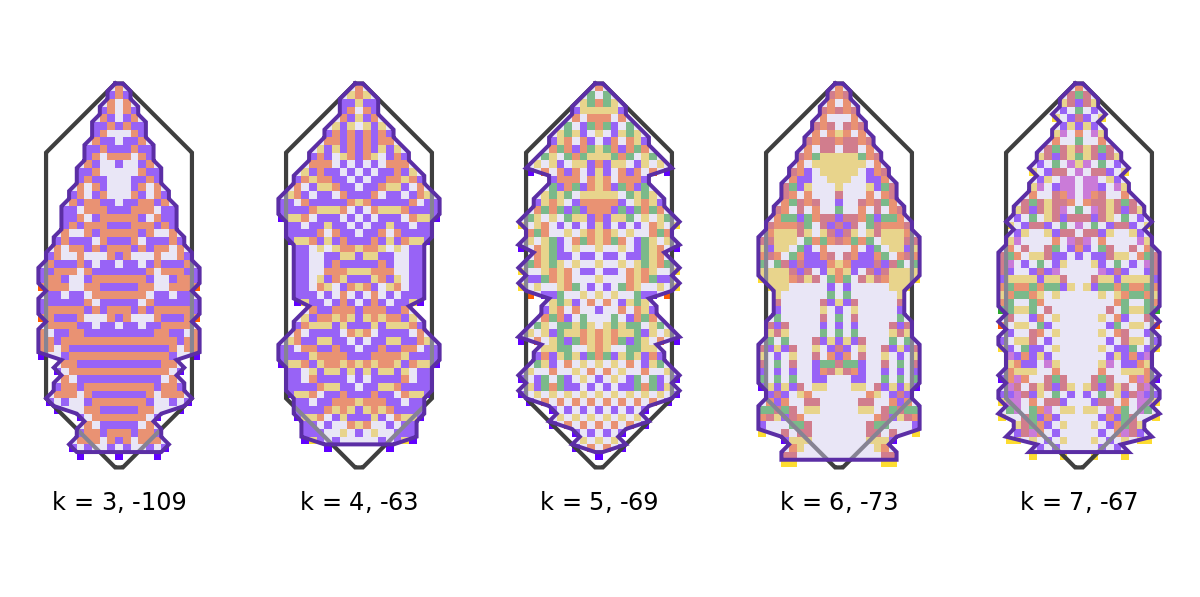
Under each cellular automata, the number of states and its fitness value is displayed. It is notable that the cases with k greater than 3 had better fitness value, but this is only the best value obtained for this “SeedRandom”, this result could be an exception and the other cases didn’t fit well. To confirm this, it is possible to analyse the mean fitness and the fitness standard variation:
Looking at the mean fitness values, it is clear that the optimal number of states so far is 5. Numbers greater than 5 did not yield a good overall result and have a greater standard deviation, indicating that this configuration can achieve great results, but they are not constant and there is a significant number of bad results. This is probably because the number of rules for k = 6 and k = 7 is much higher when compared to the other k values, which reduces the probability of selecting a single point mutation with higher fitness. The histogram plot of the fitness displayed below also suggests that the issue with higher number of states lies on the cases where the algorithm struggles to find better mutations.
One way to contour this issue and achieve better results is by performing more mutations at the same time. By doing that for k = 6, the results are:
Just from the mean fitness and the standard deviation, it is clear that adding more mutations helped improve the fitness values. Additionally, the histogram plot of the fitness value for each mutation quantity shows that more mutations have achieved better results, without getting “stuck” in a single mutation with the same fitness.
When doing the same test with 7 states, the results are similar, with the fitness values as follow:
The behaviour of the mutations histograms is also similar:
In both cases, the fitness improved as the number of mutations increased,peaking at 4 mutations for k = 6 and 5 mutations for k = 7. This suggests that there may be a limit to the fitness improvement, meaning that adding more mutations does not necessarily lead to better results.
Selecting the Best Fits
Selecting the Best Fits
Due the limited time, only a few configurations were explored in depth: k = 3, k = 4 and k = 5, all with symmetric rules and r = 1. Below, the evolution of the most relevant case found for each defined fitness function and each color count is presented.
Trying to Longer Shapes
Trying to Longer Shapes
The initial shapes showed great result, but their lifetime was between 20 and 50 steps. So, what would the evolution behavior be like for shapes with longer lifetime?
For this scenario, the shapes tested were longer versions (with 100 time steps) of those initially tested:
However, just the first shape had a great fit, following is displayed the best cases found for number of states 3, 4 and 5.
The other shapes could not evolve well and, in general, the result of the evolution was similar with the results above. In order to try different shapes, it was tested with some random shapes. Some of them got a good result, such as the following:
The failure of most shapes with longer lifetimes may be attributed to the frequency plot of the possible configurations, since the frequency of patterns with a shorter lifetime (up to 50 steps) are higher than the frequency of the shapes with more steps.
Trying to Infinite Shapes
Trying to Infinite Shapes
Tests were also conducted with infinite formats. In an effort to avoid formats that grow at a constant rate, the chosen patterns are always triangular, which forces the cellular automaton to increase its width. Some of the good results are:
Code
Code
Concluding Remarks
Concluding Remarks
This project demonstrates an analogy between the evolution of a cellular automata and fundamental principles observed in biological evolution. A key finding is that, in all the explored configurations and target shapes, the resulting format of the cellular automata consistently represents approximations of the target, rather than exactly match. This phenomenon is parallel to real biological evolution, where many of the features of organisms are the result of systemic mechanics, which reflects the computational irreducibility present in complex systems, like cellular automata.
The investigation also reveled some limitations: single-point mutations were not successful as the rule space increase (i.e., with the addition of more states). One strategy to overcome this limitation is by increasing the number of mutations applied to the cellular automaton. This approach demonstrated promising results and, with more experiments, it may led to the identification of an optimal ratio between the number of mutations and the length of the ruleset.
For future work, it is necessary to expand this study to a wider variety of target shapes and wider cellular automaton configurations. Further research could explore the optimal number of states needed to closely approximate specific target formats, as well as the ideal number of mutations required to achieve effective results with more complex rulesets.
Acknowledgments
Acknowledgments
Participating in this Summer School was a truly transformative experience and I am grateful for the opportunity to have been part of it. I extend my thanks to my family and friends for their support in this journey. I am also appreciative of the guidance and encouragement I received during the program, especially from Willem Nielsen and Alejandra Ortiz. Finally, I would like to express my deepest gratitude to Professor Pedro de Oliveira, who introduced me this world of cellular automata.
References
References
S. Wolfram (2002), A New Kind of Science. Wolfram Media.
Cite This Notebook
Cite This Notebook