Phase-Plane Analysis of Biochemical Reactors
Authors: Housam Binous and Ahmed Bellagi
Phase-Plane Analysis of Biochemical Reactors
Authors: Housam Binous and Ahmed Bellagi
Authors: Housam Binous and Ahmed Bellagi
A biochemical reactor can show complex dynamic behaviour including multiple steady - states . We show how one can obtain the different steady - states, conduct the phase - plane analysis and check for the stability of all the steady - states . Both Monod and substrate inhibition models are considered for the growth rate expression . Numerical values of yield, dilution rate, substrate concentration in the feed stream and parameters of the specific growth rate expression are the same as the treatment of B . Wayne Bequette in Process Dynamics, Modeling, Analysis and Simulation, Prentice Hall, 1998.
Reference :
Housam Binous and Ahmed Bellagi, Introducing nonlinear dynamics to chemical and biochemical engineering graduate students using MATHEMATICA©, Computer Applications in Engineering Education, 27 (1), pp . 217 - 235, 2019.
Housam Binous and Ahmed Bellagi, Introducing nonlinear dynamics to chemical and biochemical engineering graduate students using MATHEMATICA©, Computer Applications in Engineering Education, 27 (1), pp . 217 - 235, 2019.
Acknowledgement :
Numerical values were obtained from Process Dynamics, Modeling, Analysis and Simulation, B. Wayne Bequette, Prentice Hall, 1998.
Numerical values were obtained from Process Dynamics, Modeling, Analysis and Simulation, B. Wayne Bequette, Prentice Hall, 1998.
In[]:=
Off[General::"spell1"]
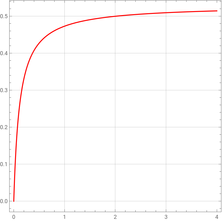
Specific growth coefficient following form proposed by Monod in 1942.
In[]:=
μ
mod
K
mod
k
mod
Out[]=
x2
K
mod
x2+
k
mod
In[]:=
K
mod
k
mod
In[]:=
plt1=Plot[,{x2,0,4},PlotStyleRGBColor[1,0,0],PlotRange->All,Frame->True,GridLines->Automatic,AspectRatio->1]
μ
mod
Out[]=
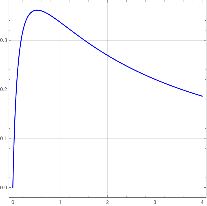
Expression of the specific growth coefficient when there is substrate inhibition.
In[]:=
μ
SI
K
SI
k
SI
k
l
Out[]=
x2
K
SI
x2++
2
x2
k
l
k
SI
In[]:=
K
SI
k
SI
k
l
In[]:=
plt2=Plot[,{x2,0,4},PlotStyleRGBColor[0,0,1],Frame->True,GridLines->Automatic,AspectRatio->1]
μ
SI
Out[]=
In[]:=
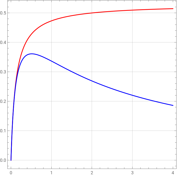
Show[plt1,plt2,PlotRange->All,Frame->True,GridLines->Automatic,AspectRatio->1]
Out[]=
Dilution rate is De=0.3; Yield is Y=0.4; x2f is the substrate concentration in the feed.
In[]:=
De=0.3;
In[]:=
Y=0.4;
In[]:=
x2f=4.0;
We find two steady-state solutions for the Monod growth rate.
In[]:=
steady1=Solve[{(-De)x10,De(x2f-x2)-x1/Y0},{x1,x2}]
μ
mod
μ
mod

Out[]=
{{x11.53739,x20.156522},{x10.,x24.}}
We find three steady-state solutions for the growth rate with substrate inhibition.
In[]:=
steady2=Solve[{(-De)x10,De(x2f-x2)-x1/Y0},{x1,x2}]
μ
SI
μ
SI
Out[]=
{{x11.53016,x20.174593},{x10.995103,x21.51224},{x10.,x24.}}
Phase-plane analysis when there is substrate inhibition in the growth rate. Red, Blue and Green dots in the figure are the three steady-states. The Red and Blue dots correspond to the stable steady-states. The Green dot is the saddle point (unstable steady-state). Only solution three (Blue dot) is non trivial. The Red dot corresponds to wash out (i.e. no biomass is left in the bioreactor).
In[]:=
μ
SI
In[]:=
μ
SI
K
SI
k
SI
k
l
In[]:=
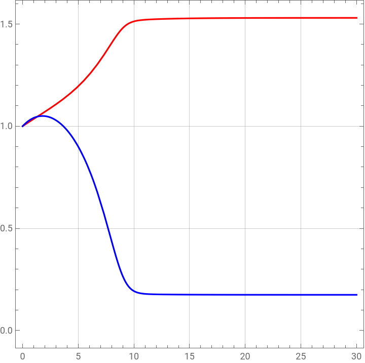
sol3=NDSolve[{D[x1[t],{t,1}]([t]-De)x1[t],D[x2[t],{t,1}]De(x2f-x2[t])-[t]x1[t]/Y,x1[0]1,x2[0]1},{x1[t],x2[t]},{t,0,30}]
μ
SI
μ
SI
Out[]=
x1[t]InterpolatingFunction[t],x2[t]InterpolatingFunction[t]


In[]:=
plt5=Plot[{Evaluate[x1[t]/.sol3],Evaluate[x2[t]/.sol3]},{t,0,30},PlotStyle{RGBColor[1,0,0],RGBColor[0,0,1]},Frame->True,GridLines->Automatic,AspectRatio->1]
Out[]=
In[]:=
sol4=NDSolve[{D[x1[t],{t,1}]([t]-De)x1[t],D[x2[t],{t,1}]De(x2f-x2[t])-[t]x1[t]/Y,x1[0]0.75,x2[0]2},{x1[t],x2[t]},{t,0,30}]
μ
SI
μ
SI
Out[]=
x1[t]InterpolatingFunction[t],x2[t]InterpolatingFunction[t]


In[]:=
tbl=Table[plt[i],{i,1,3}];
In[]:=
TBL=Table[PLT[i],{i,1,3}];
In[]:=
TbL=Table[plot[i],{i,1,15}];
In[]:=
Show[Flatten[Join[TBL,tbl,TbL,TbLx]],Graphics[{{PointSize[0.03],RGBColor[1,0,0],Point[{0,4}]},{PointSize[0.03],RGBColor[0,1,0],Point[{0.9951,1.5123}]},{PointSize[0.03],RGBColor[0,0,1],Point[{1.5302,0.1745}]}}],PlotRange->{{0,2},{0,5}},DisplayFunction$DisplayFunction]
Phase-plane analysis when the growth rate follows Monod equation. Red and Blue dots in the figure are the two steady-states. The Blue dot corresponds to the stable steady-state. The Red dot is the saddle point (unstable steady-state). Only solution two (Blue dot) is non trivial. The Red dot corresponds to wash out (i.e. no biomass is left in the bioreactor).
In[]:=
TbL=Table[plot[i],{i,1,10}];
In[]:=
Show[Flatten[Join[TbL,TbLx]],Graphics[{{PointSize[0.03],RGBColor[1,0,0],Point[{0,4}]},{PointSize[0.03],RGBColor[0,0,1],Point[{1.53739,0.15652173}]}}],PlotRange->{{0,2},{0,5}},DisplayFunction$DisplayFunction]
Stability analysis when the growth rate follows Monod equation. We look at the signs of the eigenvalues of the Jacobian Matrix. Steady-state (0,4) is unstable because eigenvalues are of opposite sign indicating that it is a saddle point. Steady-state (1.53739,0.156522) is a stable steady-state because both eigenvalues are negative.
Stability analysis when the growth rate is subject to substrate inhibition. We look at the signs of the eigenvalues of the Jacobian Matrix. Steady-states (0,4) and (1.53016,0.174593) are both stable because their eigenvalues are negative. Steady-state (0.995103,1.51224) is a saddle point because its eigenvalues have opposite signs.