To celebrate once more the glorious π day! Here it goes more π visualization!
Pi is a symbolic expression in Wolfram Language:
In[]:=
Pi
Out[]=
π
Little help info about Pi function:
In[]:=
?Pi
Out[]=
And some definition from Wikipedia:
In[]:=
CellPrint[TextCell[#,"CodeText"]&/@TextSentences[WikipediaData["Pi"]][[;;6]]]
The number π (; spelled out as "pi") is a mathematical constant that is the ratio of a circle's circumference to its diameter, approximately equal to 3.14159.
The number π appears in many formulae across mathematics and physics.
It is an irrational number, meaning that it cannot be expressed exactly as a ratio of two integers, although fractions such as
22
7
7
{\displaystyle {\tfrac {22}{7}}}
are commonly used to approximate it.
are commonly used to approximate it.
Consequently, its decimal representation never ends, nor enters a permanently repeating pattern.
You can get any numerical precision you wanted:
In[]:=
N[Pi,100]
Out[]=
3.141592653589793238462643383279502884197169399375105820974944592307816406286208998628034825342117068
The first 1000 primes in π
In[]:=
N[Pi,1000]
Out[]=
3.141592653589793238462643383279502884197169399375105820974944592307816406286208998628034825342117067982148086513282306647093844609550582231725359408128481117450284102701938521105559644622948954930381964428810975665933446128475648233786783165271201909145648566923460348610454326648213393607260249141273724587006606315588174881520920962829254091715364367892590360011330530548820466521384146951941511609433057270365759591953092186117381932611793105118548074462379962749567351885752724891227938183011949129833673362440656643086021394946395224737190702179860943702770539217176293176752384674818467669405132000568127145263560827785771342757789609173637178721468440901224953430146549585371050792279689258923542019956112129021960864034418159813629774771309960518707211349999998372978049951059731732816096318595024459455346908302642522308253344685035261931188171010003137838752886587533208381420617177669147303598253490428755468731159562863882353787593751957781857780532171226806613001927876611195909216420199
One easy (low cost computation) and popular π approximation is 22/7:
In[]:=
22/4
Out[]=
11
2
In[]:=
N[22/7]
Out[]=
3.14286
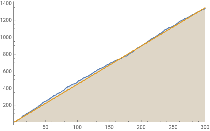
We can compare both π and the approximation 22/7, accumulating then for their first 300 digits:
ListLinePlot[{Accumulate[First[RealDigits[N[Pi,300]]]],Accumulate[First[RealDigits[N[22/7,300]]]]},FillingAxis,PlotLegends{"π","22/7"}]
Out[]=


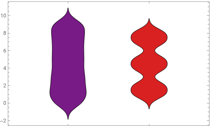
We can compare the first 1000 digits of π and 22/7 with a distribution chart. It illustrates the correlation between quantitative data points for distribution analysis.
In[]:=
DistributionChart[{First[RealDigits[N[Pi,1000]]],First[RealDigits[N[22/7,1000]]]},ChartStyle"Rainbow",ChartLegends{"π","22/7"}]
Out[]=


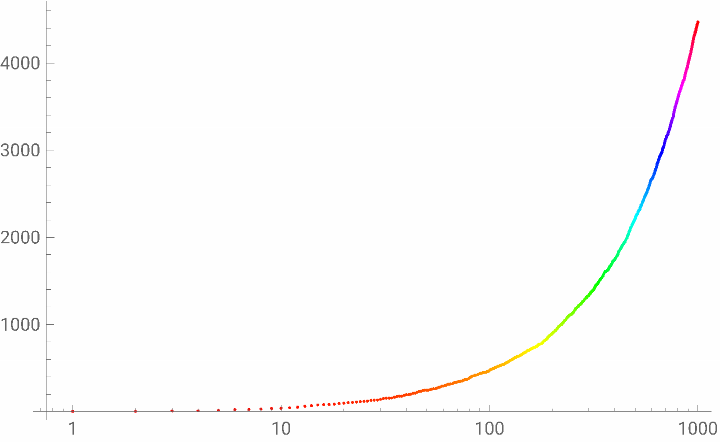
Log view of accumulating the π digits up to 1000 first:
In[]:=
ListLogLinearPlot[Accumulate[First[RealDigits[N[Pi,1000]]]],ColorFunction->Hue]
Out[]=
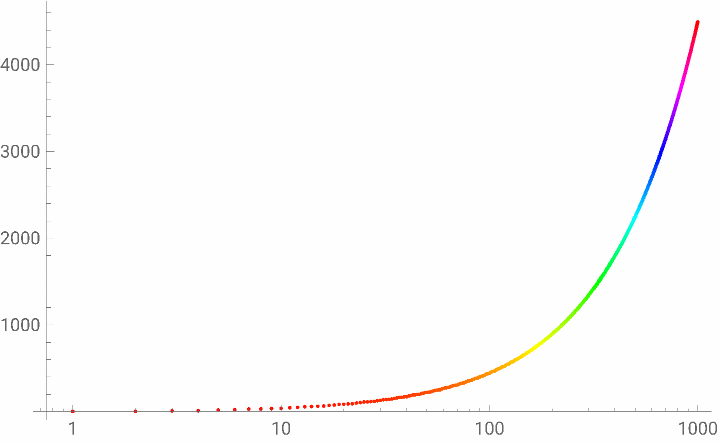
And the log view of accumulating the 22/7 approximation digits up to 1000 first :
In[]:=
ListLogLinearPlot[Accumulate[First[RealDigits[N[22/7,1000]]]],ColorFunction->Hue]
Out[]=
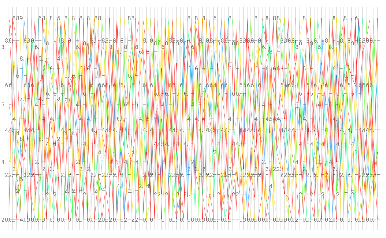
Now we can break the 1000 first digits by 100 and view side by side in a ParallelAxisPlot, it sounds pretty random:
In[]:=
ParallelAxisPlot[Partition[First[RealDigits[N[Pi,1000]]],100],ColorFunction->Hue,ColorFunction->"Rainbow"]
Out[]=
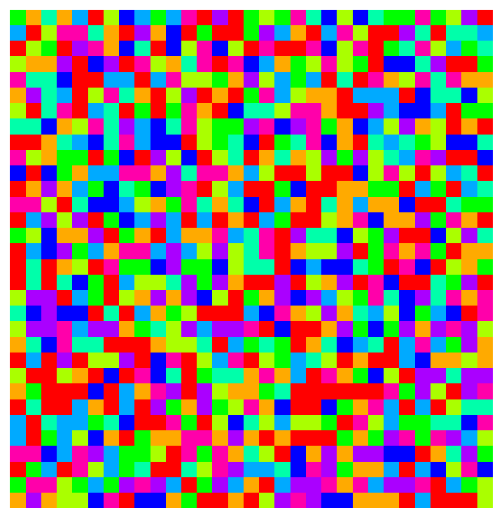
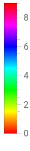
Lets create a 2D image for the first 1000 digits, when we color it according the digit values from 0 to 9:
In[]:=
piData=Partition[First[RealDigits[N[Pi,1000]]],Floor[Sqrt[1000]]];ArrayPlot[piData,ColorFunction->Hue,PlotLegendsAutomatic,Frame->None]
Out[]=
We can calculate the numerical Fourier and view the imaginary, absolute and real digits plots...
In a pie chart we can notes that the distribution is really close for each digit as we go...
It is interesting to view the order when the digits first appears at the π sequence:
And finally visualize the π digits in a elegant Chord Diagram:
This Chord Diagram shows, for the first 100 digits of π sequence, what is the next digit case. Notes that 9 goes most to 7 and 8 as the next digits.
Growing the number of π digits to ∞, the graphic wound gets more homogeneous.
Gettring it all toghether we can have a interactive visualization for π digits at the Chord Diagram:
π is fun! Explore more about π with Wolfram Language! Enjoy!