Preamble
Preamble
We will apply a technique from control theory to the case of a damped harmonic oscillator in one spatial dimension. Specifically, we would like to specify a time-dependent external force in just such a way that a damped harmonic oscillator evolves to some fixed position away from the minimum of the potential well.
The technique we will discuss today, known as Proportional-Integral-Derivative (PID) control, although not often taught as a part of the standard theoretical physics curriculum, is nevertheless interesting when considered from a theoretical physics perspective as well. (For an in depth treatment of the problem of control, I refer readers to Russ Tedrake’s excellent lecture notes on Underactuated Robotics from MIT [ https://underactuated.csail.mit.edu/ ].)
In the time-honored physicist tradition, we will learn the basics of the technique by applying it to the simple harmonic oscillator, and as we will see, this will make the logic of the PID control technique quite transparent.
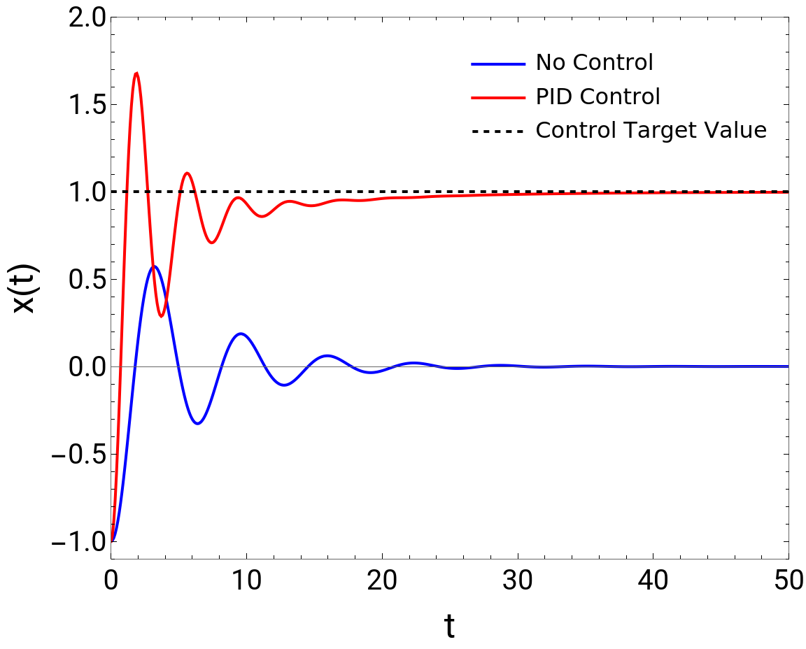
Figure: The result of applying PID control to a damped simple harmonic oscillator. In the absence of control the particle undergoes a decaying oscillation until it comes to rest at the minimum of the potential at (blue curve). In the presence of our “control” force, the particle can be made to stably occupy some position away from the potential minimum (red curve).
x=0
Equations of Motion
Equations of Motion
We will consider the case of a damped harmonic oscillator subject to an external force where γ is the drag coefficient, and is the natural frequency of the harmonic oscillator.We next specify how we wish to “control” our oscillator. For simplicity, we will try to force the particle to sit at some fixed position ≠0. (Obviously, the equilibrium position of the oscillator will be after a sufficiently long time in the absence of driving force .)For PID control, we introduce the error function and then the “control function” or external driving force will take the form . The driving force consists of three terms, one (P)roportional to the error, one which goes as the (I)ntegral of the error, and one which goes as the (D)erivative of the error, hence “PID.” Note that we have introduced three parameters ,, here, and in many real-world applications the determination of these parameters is the crucial step of the problem, and will dictate the quality of your controller. As we shall see below, for our problem adequate values can be easily found by trial and error. At the end of the post I will return to the question of how to determine these parameters in the case where trial and error is insufficient.
u(t)
x''(t)+γx'(t)+x(t)=u(t)
2
ω
ω
*
x
x=0
u(t)
e(t)=-x(t)
*
x
u(t)=e(t)++e(t')dt'
K
p
K
d
de(t)
dt
K
i
t
∫
0
K
p
K
d
K
i
For now, we are in familiar territory as physicists, as we have expressed our control problem as the solution of an equation, in this case a second order linear integrodifferential equation. Solving it (at least numerically) is not as bad as it sounds.First though, we plug in, and we obtain . Already, the structure of this equation reveals something interesting. We see that the parameter acts just like another drag coefficient, and the parameter acts like another spring force, although in this case the force does not pull the particle back to the origin, but instead towards our target position . Thus, the effect of the proportional and derivative terms in our PID driving force is to act like a damped harmonic oscillator, but one whose equilibrium position is at the desired target position rather than the minimum of the original potential well. Of course, in the absence of other forces, our system would now spontaneously evolve towards the target position! This is starting to feel like control.The final term is slightly more unusual. It acts like a memory-dependent force, whose value depends on the entire history of the system, rather than its instantaneous state. One encounters forces like this in equations of motion for non-Markovian stochastic processes (see, for example, Zwanzig, Nonequilibrium Statistical Mechanics, Chapter 1), where they sometimes instead involve integrals over the particle’s velocity history rather than its position history. The appearance of such memory-dependent forces is an interesting consequence of applying the PID framework to this simple system.
x''(t)+(γ+)x'(t)++x(t)--(-x(t'))dt'=0
K
d
2
ω
K
p
K
p
*
x
K
i
t
∫
0
*
x
K
d
that
K
p
*
x
-(-x(t))dt
K
i
t
∫
0
*
x
Numerical Solution of the Equations of Motion
Numerical Solution of the Equations of Motion
We now wish to numerically solve the equations of motion for this problem. To do so, we will convert our second order equation into a system of first order equations by introducing new variables (t)=(-x(t'))dt' (t)=x(t)(t)=x'(t)
x
0
t
∫
0
*
x
x
1
x
2
Upon substitution, our equations of motion become
=
+
. Linear inhomogeneous differential equations of this type have a general solution which is given by '(t)=A(t)+⟹ (t)=exp(At)+exp(At)exp(-At')dt' . (Source: Boas, Mathematical Methods in the Physical Sciences, Chapter 8.) Thus, provided we can exponentiate the matrix in our equation above, we can calculate the time evolution of our system. At this point, finding an analytical solution would require exponentiating the matrix above symbolically, which is tricky to do, so we choose to proceed numerically instead. Lucky for us, Wolfram Language has the “MatrixExp[]” function which handles the matrix exponentiation nicely. (If you are partial to Python, you can use scipy.linalg.expm() function instead.)
d
dt
x 0 |
x 1 |
x 2 |
0 | -1 | 0 |
0 | 0 | 1 |
K i | - 2 ω K p | -(γ+ K d |
x 0 |
x 1 |
x 2 |
* x |
0 |
* x K p |
x
x
b
x
x
0
t
∫
0
b
We now choose some numerical values for the drag, oscillator frequency, and target position, and perform the integral to determine the time dependence.
(*Parameters*)Clear[Ki,Kp,Kd,A,b,x0,xt,fspring,fdrag,up,ud,ui];gamma=0.35;w02=1.0;xbar=1.0;Ki=0.3;Kp=2.0;Kd=0.4;(*Times*)ts=Range[0.,50.,0.1];Δt=ts[[2]]-ts[[1]];A={{0.,-1.,0.},{0.,0.,1.},{Ki,-w02-Kp,-gamma-Kd}};b={xbar,0,xbar*Kp};(*Initialcondition*)x0={0.,-1.,0.};(*Storagearrays*)xt=ConstantArray[0.,Length[ts]];fspring=ConstantArray[0.,Length[ts]];fdrag=ConstantArray[0.,Length[ts]];up=ConstantArray[0.,Length[ts]];ud=ConstantArray[0.,Length[ts]];ui=ConstantArray[0.,Length[ts]];Do[(*Matrixexponentialforcurrenttime*)statet=MatrixExp[A*ts[[i]]].x0;(*KernelintegralapproximationbyRiemannsum*)kern=Total[Table[MatrixExp[-A*ts[[j]]],{j,1,i}]];kern=kern*Δt;statet=statet+MatrixExp[A*ts[[i]]].kern.b;(*Recordforcesandcontrolterms*)fspring[[i]]=-w02*statet[[2]];fdrag[[i]]=-gamma*statet[[3]];up[[i]]=Kp*(xbar-statet[[2]]);ud[[i]]=-Kd*statet[[3]];ui[[i]]=Ki*statet[[1]];xt[[i]]=statet[[2]];,{i,Length[ts]}];(*Nowxt,fspring,fdrag,up,ud,uiholdthetrajectories*)
Regardless of what initial position and velocity we give our particle, the control algorithm always robustly directs it to the target steady-state position.
It is also instructive to examine the individual forces which sum to determine the particle’s motion.
We observe several interesting aspects of the evolution of these forces. At early times, the proportional term from the controller is the largest in magnitude, followed by the spring force. We observe that the drag force and the derivative term from the controller are almost identical in their contributions. Finally, at long times, when the mass is no longer moving, and its position lies very near the target position, so that the drag, derivative, and proportional force terms vanish, it is the integral term which serves to counterbalance the restoring force of the spring and hold the particle in place.
Concluding Remarks
Concluding Remarks
CITE THIS NOTEBOOK
CITE THIS NOTEBOOK
Proportional-integral-derivative control of a simple harmonic oscillator
by Matthew Kafker
Wolfram Community, STAFF PICKS, September 22, 2025
https://community.wolfram.com/groups/-/m/t/3548805
by Matthew Kafker
Wolfram Community, STAFF PICKS, September 22, 2025
https://community.wolfram.com/groups/-/m/t/3548805